How can you Create and Customize Heat Maps in Excel?
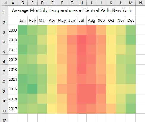
Creating heat maps in Excel is a great way to visualize data trends and patterns, helping you make data-driven decisions efficiently. This step-by-step guide will walk you through the process of creating and customizing heat maps in Excel.
Step 1: Open Microsoft Excel and Enter Your Data
- Open Microsoft Excel on your computer.
- Enter your dataset into a new worksheet. Make sure your data is organized in rows and columns for easy analysis.
Step 2: Select the Data Range
- Click and drag your mouse over the cells containing your data to select the entire range, including headers.
Step 3: Apply Conditional Formatting
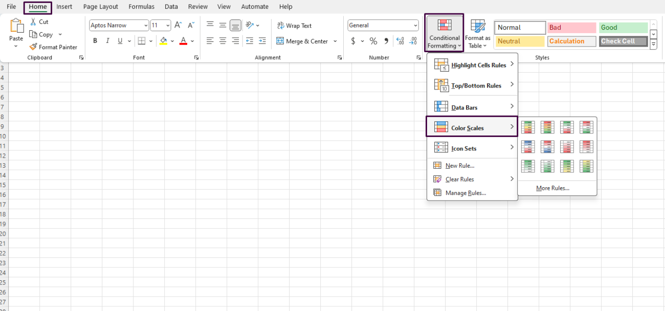
Navigate to the Home tab on the Ribbon.
- Click on
Conditional Formattingin the Styles group. - Hover over
Color Scalesto see a variety of color gradient options. - Choose a color scale that best represents your data (e.g., Green-Red Color Scale).

Step 4: Customize the Color Scale Conditional Formatting
- After applying the color scale, click on
Conditional Formattingagain. - Select
Manage Rulesfrom the drop-down menu. - In the Conditional Formatting Rules Manager dialog box, make sure your current worksheet is selected.
- Click on the rule you applied and then click
Edit Rule.
Step 5: Modify the Rule’s Settings
- Within the Edit Formatting Rule dialog box, you’ll see the
Format Styleset to Color Scale. - Customize the color scale by setting the
Minimum,Midpoint, andMaximumvalues, and their corresponding colors.- Example:
- Minimum:
2-Color Scale- Value: Number, 0
- Color: Blue
- Maximum:
2-Color Scale- Value: Number, 220 (or adjust based on your dataset)
- Color: Red
- Minimum:
- Example:
- Click
OKafter making your adjustments. - Click
Applyand thenOKto close the dialog box.
Step 6: Fine-tune Your Heat Map
- Adjust the cell sizes to ensure the heat map is easily readable:
- Click and drag the column and row headers to resize the cells.
- Optionally, add data labels for better clarity:
- Right-click on the formatted cells and select
Format Cells. - Go to the
Numbertab. - Choose
Numberor any other appropriate format to display data clearly.
- Right-click on the formatted cells and select

Step 7: Save and Share Your Heat Map
- Save your Excel workbook to prevent loss of data:
- Go to
File>Save Asand select the file location and format.
- Go to
- Share your heat map with others by either emailing the file or exporting it as a PDF:
- To export as PDF, go to
File>Save As, choose PDF from the file type dropdown menu, and clickSave.
- To export as PDF, go to
Unlock incredible deals on Office Keys at the lowest prices available exclusively on our website!

