How do I Create a Drop-down List in Excel?
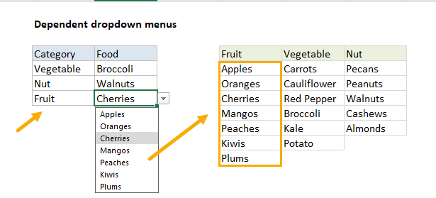
Drop-down lists in Excel are a valuable tool for enhancing the user experience and ensuring consistency when working with data. A drop-down list allows users to select a value from a predefined list, significantly reducing the chances of making mistakes during data entry. Using drop-down lists in Excel can not only simplify data entry but also improve the accuracy and organization of the information. In this guide, we will outline step-by-step instructions on how to create a drop-down list in Excel, highlighting its benefits and demonstrating how it can enhance your work with spreadsheets.
Creating a drop-down list in Excel is a straightforward process that can be completed in just a few simple steps. By first creating a list of values and then defining the cell range, users can easily create a drop-down list within their Excel sheet. This feature is particularly effective when working with large datasets, eliminating the need for manual entry and minimizing the likelihood of errors.
Step 1: Open Microsoft Excel
Start by opening Microsoft Excel on your computer. Locate the Excel icon in the Start menu or search for “Excel” in the search bar.
Step 2: Create or Open a Workbook
Create a new workbook by selecting “File” from the top menu and choosing “New” from the dropdown menu. Alternatively, open an existing workbook by selecting “Open” and browsing to the desired file location.
Step 3: Select the Cell Range
Choose the range of cells where you want to create the drop-down list. For example, select cells A1:A5 to create a list in column A.
Step 4: Open the Data Validation Menu
From the top menu, select the “Data” tab, and then click on the “Data Validation” button. This will open the Data Validation dialog box.
Step 5: Choose the Validation Criteria
In the Data Validation dialog box, select “List” from the “Allow” dropdown menu.
Step 6: Specify the Source of the List
In the “Source” field, you can enter the values manually, separated by commas. For example, you can type “Apple, Banana, Cherry, Orange” directly in the Source field.
Alternatively, you can refer to a range of cells where you have already entered the desired values. To do this, click on the cell range icon next to the Source field, and then select the cells containing the values for your drop-down list.

Step 7: Customize the Error Alert (Optional)
If you want to display an error alert when someone enters an invalid value in the drop-down list, go to the Error Alert tab in the Data Validation dialog box. You can customize the error message and choose the error style.
Step 8: Test the Drop-down List
Once you have set the validation criteria and specified the source of the list, click “OK” to close the Data Validation dialog box. You should now have a drop-down arrow in the selected cell range. Clicking the arrow will display the values from your list.
Step 9: Copy the Drop-down List (Optional)
If you want the drop-down list to appear in other cells, simply copy the cell range (containing the drop-down list) and paste it in the desired cells.
Step 10: Save and Share Your Workbook
After creating the drop-down list, remember to save your workbook by selecting “File”, then “Save”. You can also share your workbook with others by selecting “File”, “Share”, and following the prompts.
By following these step-by-step instructions, you can easily create a drop-down list in Microsoft Excel, making data entry more efficient and ensuring consistency.
Get the power of Microsoft Office at the lowest price on our website, unlocking premium productivity tools for your personal and professional needs.

