How do you Find and Highlight Blank Cells in Excel?

Microsoft Excel is a powerful tool for data analysis and management. One common task is identifying and highlighting blank cells within a dataset. Blank cells can disrupt data integrity, making it important to locate and address them quickly. In this blog post, we’ll walk you through step-by-step instructions on how to find and highlight blank cells in Excel.

Step 1: Open Your Excel Workbook

1. Launch Microsoft Excel.
2. Open the workbook that contains the dataset you want to inspect.

Step 2: Select the Range of Cells

1. Click on the top-left cell of the range you want to check.
2. Drag the cursor to cover the entire range, or use keyboard shortcuts:
   • Press Ctrl + A to select the entire worksheet.
   • Hold down Shift and press the arrow keys to select a custom range.

Step 3: Open the “Go To Special” Dialog Box

1. Navigate to the Home tab on the ribbon.
2. Click on Find & Select in the Editing group.
3. Select Go To Special from the dropdown menu.

Alternatively, you can press Ctrl + G and then click on Special.

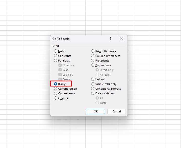
Step 4: Select “Blanks” in the “Go To Special” Dialog Box

1. In the Go To Special dialog box, select the Blanks option.
2. Click OK. Excel will now highlight all blank cells in the selected range.

Step 5: Highlight the Blank Cells

1. With the blank cells still selected, go back to the Home tab.
2. In the Font group, click on the Fill Color button (paint bucket icon).
3. Choose a color to fill the blank cells.

Step 6: Verify the Highlighted Cells

Ensure that all blank cells are appropriately highlighted. Scroll through the dataset to double-check if necessary.

Step 7: Save Your Workbook

1. Click on File.
2. Select Save or Save As and choose a location to store your updated workbook.

Unlock the full potential of your productivity by purchasing the cheapest Office Keys available, offering all the features you need at an unbeatable price.