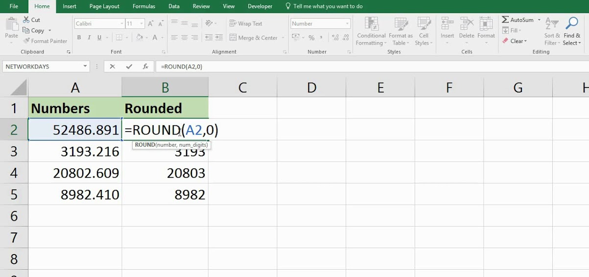
How to use the ROUNDUP Function in Excel?

Using the ROUNDUP function in Excel is a straightforward way to round numbers up to a specified number of decimal places or to the nearest whole number. This guide will walk you through the process step-by-step, with specific commands for each part of the process.

Step 1: Open Your Excel File

1. Launch Excel: Start Microsoft Excel on your computer.
2. Open an Existing Workbook or Create a New One: Go to “File” > “Open” to browse for an existing workbook or “File” > “New” to create a new one.
3. Select the Worksheet: Navigate to the worksheet where you want to use the ROUNDUP function.

Step 2: Identify the Number to Round Up

1. Locate the Number: Find the cell that contains the number you intend to round up. This will usually be in a column of data.
2. Check the Number: Ensure the number is in numerical format for the ROUNDUP function to work properly.

Step 3: Select the Destination Cell for the ROUNDUP Function

1. Choose Target Cell: Click on the cell where you want the rounded-up value to appear (e.g., if your original number is in cell A1, you might use cell B1 for the ROUNDUP function).

Step 4: Enter the ROUNDUP Function

1. Activate Formula Mode: In your target cell, start by typing an equals sign = to enter formula mode.
2. Type ROUNDUP: Begin typing ROUNDUP( to initiate the function.
3. Add Number Reference: Click on the cell with the number you want to round up (e.g., A1) to add it to the formula, or manually type A1.
4. Specify Number of Digits: Type a comma , followed by the number of decimal places to which you want to round up (e.g., 2 for two decimal places). Your formula should look like this: =ROUNDUP(A1, 2).
5. Close Parenthesis: Type a closing parenthesis ) to complete the formula.
6. Press Enter: Hit Enter on your keyboard to execute the function.

Step 5: Round Up to the Nearest Integer (If Needed)

1. Activate Formula Mode Again: In your target cell, start by typing an equals sign = to enter formula mode.
2. Type ROUNDUP: Begin typing ROUNDUP( to initiate the function.
3. Add Number Reference: Click on the cell with the number you want to round up (e.g., A2) to add it to the formula, or manually type A2.
4. Specify Zero Decimal Places: Type a comma , followed by 0 to round to the nearest integer. Your formula should look like this: =ROUNDUP(A2, 0).
5. Close Parenthesis: Type a closing parenthesis ) to complete the formula.
6. Press Enter: Hit Enter on your keyboard to execute the function.

Step 6: Copy the Formula to Adjacent Cells (If Needed)

1. Select the Formula Cell: Click on the cell with the ROUNDUP function (e.g., B1).
2. Drag the Fill Handle: Hover over the bottom-right corner of the cell until you see a small ‘+‘ sign. Click and drag down or across to copy the formula to adjacent cells.
3. Release Mouse Button: Release the mouse button when you have covered all the necessary cells. Excel will auto-update the formulas to reference the corresponding number cells.

Step 7: Check and Verify Your Results

1. Review Rounded Values: Ensure that the rounded values are correct and meet your expectations.
2. Adjust If Necessary: If the rounded values do not appear as expected, verify that the original data is accurate and that the formula was entered correctly.

Step 8: Save Your Workbook

1. Save Your Work: Click on “File” > “Save” or press Ctrl + S to save the existing workbook.
2. Save As New Version: If you want to preserve the original data, select “File” > “Save As” and create a new version of your workbook.

Get genuine Office Keys at unbeatable prices on cheapkeys.io – your ultimate destination for affordable software solutions!