What is the use of Slicers in PivotTables in Excel?

In the world of data analysis and reporting, Excel’s PivotTables are indispensable tools. They allow users to efficiently summarize, analyze, explore, and present complex datasets. Among the many features available to enhance PivotTables, Slicers stand out as particularly powerful. This blog explores the use of Slicers in PivotTables, explaining what they are, their benefits, and how to use them effectively.

Understanding Slicers

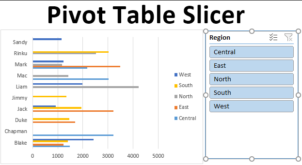
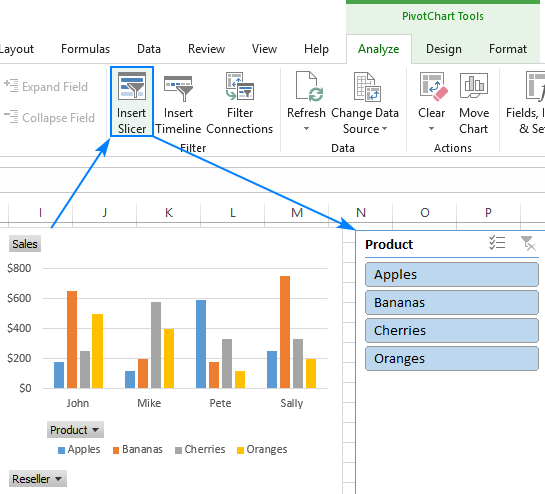
Slicers are visual filters that make it easier to dynamically filter data in PivotTables. Introduced in Excel 2010, Slicers provide a user-friendly interface for filtering that is both intuitive and interactive. Instead of using the traditional drop-down filters within PivotTables, Slicers display filter buttons that users can click to filter the data.

The Benefits of Using Slicers

1. Enhanced User Experience

• Visual Clarity: Slicers offer a visually distinct and appealing way to filter data, enhancing the overall user experience.
• Ease of Use: With just a few clicks, users can quickly filter data without navigating complex menus.

2. Improved Data Analysis

• Immediate Updates: Slicers allow for real-time updates to PivotTables, enabling users to see the effects of different filters instantly.
• Cross-Compatibility: Slicers can be used to filter multiple PivotTables simultaneously, making it easier to compare different datasets.

3. Professional Reporting

• Polished Appearance: Slicers add a professional touch to reports, making them more engaging and easier to understand.
• Customizable: Slicers can be customized in terms of size, style, and layout, allowing them to perfectly match the aesthetics of your report.

How to Use Slicers in PivotTables

Step 1: Create a PivotTable

1. Select your data range.
2. Go to the Insert tab on the Ribbon.
3. Click on PivotTable and follow the prompts to create your PivotTable.

Step 2: Insert a Slicer

1. Click anywhere within the PivotTable.
2. Go to the PivotTable Analyze (or Analyze in older versions) tab on the Ribbon.
3. Click on Insert Slicer.
4. A dialog box will appear. Select the fields you want to use as filters and click OK.

Step 3: Filter Your Data

• Click on the buttons within the Slicer to filter your PivotTable data.
• To select multiple items, hold down the Ctrl key while clicking.

Step 4: Customize Your Slicer

• Resize: Drag the edges of the Slicer to resize it.
• Style: Use the Slicer Tools options on the Ribbon to change the style and color of the Slicer.
• Settings: Right-click on the Slicer and choose Slicer Settings to further customize its behavior and appearance.

Practical Applications of Slicers

1. Sales Performance Analysis

• Quickly filter sales data by region, product category, or salesperson to identify trends and performance metrics.

2. Financial Reporting

• Use Slicers to dynamically filter financial reports by time periods, departments, or expense categories, making budget reviews more efficient.

3. Project Management

• Filter project timelines and tasks by status, assigned team member, or project phase to better manage and report on project progress.

Unlock the full potential of your productivity by purchasing genuine Office Keys from our website, ensuring you receive the best in office software solutions.