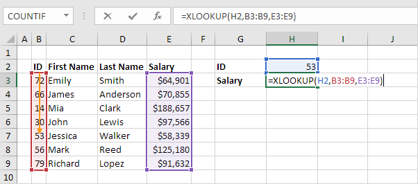
How can you use the XLOOKUP Function in Excel?

Microsoft Excel’s XLOOKUP function is a powerful tool that allows users to search for a value within a range or array and return a corresponding value from another range or array. This function is more versatile than its predecessors, VLOOKUP and HLOOKUP, and can help you streamline complex data analysis tasks.

In this blog post, we will walk you through a step-by-step guide on how to use the XLOOKUP function effectively.

Step 1: Understanding the XLOOKUP Function Syntax

The basic syntax for the XLOOKUP function is as follows:

XLOOKUP(lookup_value, lookup_array, return_array, [if_not_found], [match_mode], [search_mode])

• lookup_value: The value you are searching for.
• lookup_array: The range or array to search within.
• return_array: The range or array to return the value from.
• [if_not_found] (optional): The value to return if no match is found.
• [match_mode] (optional): Specifies the type of match (e.g., exact, wildcard).
• [search_mode] (optional): Specifies the search mode (e.g., first-to-last, last-to-first).

Step 2: Preparing Your Data

Before you can use the XLOOKUP function, you need to have your data organized. Make sure you have:

1. A lookup table where you can search for values.
2. A return table from which you can retrieve corresponding values.

For example, if you have a list of employee IDs (lookup values) and their names (return values), make sure they are aligned in a clear and structured manner.

Step 3: Entering the XLOOKUP Formula

1. Select the cell where you want the result to appear.
2. Begin typing the formula: Start with =XLOOKUP(.
3. Enter the lookup value: Type the reference to the cell containing the value you are searching for. For example, A2.
4. Specify the lookup array: Type the range or array where you expect to find the lookup value, such as B2:B100.
5. Define the return array: Enter the range or array from which you want to return the result, like C2:C100.

Your formula should now look something like this:

=XLOOKUP(A2, B2:B100, C2:C100)

Step 4: Adding Optional Parameters

To make your XLOOKUP function more robust, you can add optional parameters:

1. [if_not_found]: Specify what to return if there is no match. For example, "Not Found" can be used.

=XLOOKUP(A2, B2:B100, C2:C100, "Not Found")

2. [match_mode]: Determine the type of match you need (0 for exact match by default, 1 for next larger, -1 for next smaller, 2 for wildcard). For an exact match:

=XLOOKUP(A2, B2:B100, C2:C100, "Not Found", 0)

3. [search_mode]: Set the search mode (1 for first-to-last by default, -1 for last-to-first, 2 for binary search ascending, -2 for binary search descending). For searching from last-to-first:

=XLOOKUP(A2, B2:B100, C2:C100, "Not Found", 0, -1)

Step 5: Applying the Formula

1. Press Enter to complete the formula.
2. Drag the fill handle (small square at the bottom-right of the selected cell) to copy the formula to other cells, if needed.

Step 6: Testing and Verifying

Finally, it’s crucial to test and verify your XLOOKUP function:

1. Check different lookup values to ensure they return the correct results.
2. Verify edge cases like non-existent lookup values to confirm the [if_not_found] parameter works correctly.
3. Validate the match and search modes according to your data requirements.

Unlock the full potential of your productivity by purchasing genuine Office Keys from our website, ensuring you receive the best in office software solutions.