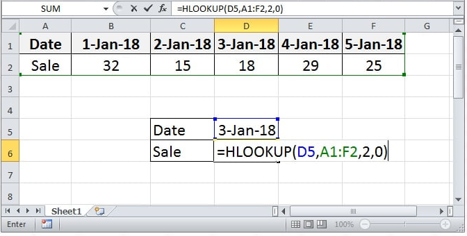
How do you use the HLOOKUP Function in Excel?

The HLOOKUP function in Excel is a powerful tool that allows you to search for a value in the top row of a table or range and return a value in the same column from a row you specify. Here’s a step-by-step guide to using the HLOOKUP function effectively.

Step 1: Understand the Syntax

Before diving into using the HLOOKUP function, it’s important to understand its syntax:

HLOOKUP(lookup_value, table_array, row_index_num, [range_lookup])

• lookup_value: The value you want to find in the top row of the table.
• table_array: The range of cells that contains the value you want to find.
• row_index_num: The row number in the table from which to retrieve the value.
• range_lookup (optional): A Boolean value (TRUE or FALSE) that specifies whether you want an exact match (FALSE) or an approximate match (TRUE).

Step 2: Set Up Your Data

Ensure your data is organized in a horizontal table format, with labels in the first row.

Step 3: Enter the HLOOKUP Formula

1. Select the cell where you want the result of the HLOOKUP function to appear.
2. Begin typing the formula by entering =HLOOKUP(.

Example:

Suppose you want to find the revenue for the month of February.

3. In cell F1, type the following formula:

=HLOOKUP("February", A1:D3, 2, FALSE)

Here’s the breakdown:

• “February”: This is the value you are searching for in the first row.
• A1:D3: This is the range of your table.
• 2: This indicates that you want the value from the second row of the table.
• FALSE: This ensures you’re looking for an exact match.

4. Press Enter. If done correctly, cell F1 will display 12000.

Step 4: Handling Approximate Matches

If you want to find the nearest match, you can use the range_lookup argument as TRUE or omit it entirely since TRUE is the default.

Example:

=HLOOKUP("Feb", A1:D3, 2, TRUE)

This will search for the closest match to “Feb” if an exact match is not found.

Step 5: Use Named Ranges for Clarity

For better readability and manageability, you can name your range. For example, select A1:D3, and in the Name Box (left of the formula bar), type Data_Table. Now, update your formula:

=HLOOKUP("February", Data_Table, 2, FALSE)

Step 6: Error Handling

If HLOOKUP cannot find the lookup_value, it will return an #N/A error. To handle this, use the IFERROR function:

=IFERROR(HLOOKUP("February", Data_Table, 2, FALSE), "Not Found")

This formula will return “Not Found” if the value is not available in the table.

Unlock the full potential of your productivity by purchasing genuine Office Keys from our website, ensuring you receive the best in office software solutions.