How can you Analyze Survey Data in Excel?
Analyzing survey data in Excel allows you to organize, visualize, and interpret your findings effectively. Follow these detailed steps to analyze your survey data using Excel.
Step 1: Import Survey Data into Excel
- Launch Microsoft Excel on your computer.
- Open a new workbook by clicking
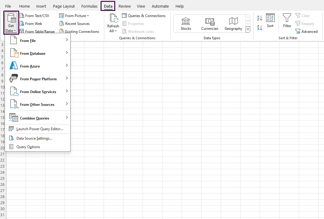
File>New. - Import your survey data by clicking
Data>Get Data(orFrom Text/CSV,From Web, etc., depending on your data source). - Follow the prompts to import your data and load it into the Excel workbook.

Step 2: Clean Your Data
- Go through your data to identify any incomplete or incorrect entries.
- Use the
Find & Selectfunction to locate blanks or errors (Home>Find & Select>Go To Special> selectBlanksorFormulas). - Correct or remove erroneous data entries and fill in any missing information as needed.
Step 3: Organize Your Data into Tables
- Select the range of your survey data.
- Go to the
Inserttab and clickTable. - Ensure the checkbox for
My table has headersis checked and clickOKto create a table.
Step 4: Use Formulas for Initial Analysis
- Use functions like
AVERAGE,MEDIAN,MODE,COUNTIF, andSUMIFto calculate basic statistics. - For example, to calculate the average of responses in column B: enter
=AVERAGE(B:B)in an empty cell. - Use
COUNTIF(range, criteria)to count occurrences of specific responses.
Step 5: Create Pivot Tables for Deeper Insights
- Click anywhere within your data table, then go to the
Inserttab and selectPivotTable. - Choose where you want the PivotTable report to be placed (New Worksheet or Existing Worksheet) and click
OK. - In the PivotTable Field List, drag and drop fields to the
Rows,Columns,Values, andFiltersareas to summarize your data.
Step 6: Visualize Data with Charts
- Select the data range you want to visualize.
- Go to the
Inserttab and choose from various charts likeColumn Chart,Pie Chart, orBar Chart. - Customize your chart using
Chart Toolsfor titles, labels, and styles.
Step 7: Use Conditional Formatting
- Highlight the range of data you want to format.
- Go to the
Hometab and selectConditional Formatting. - Choose a rule type like
Color Scales,Data Bars, orIcon Setsto highlight patterns within your data.
Step 8: Summarize Findings with Insights
- In a new worksheet, summarize key findings from your analysis.
- Use
Text BoxesandLink Cells(Insert>Text Box) to present data highlights. - Create a dashboard summarizing key statistics, visualizations, and insights for easy reference.
Step 9: Review and Save Your Workbook
- Review your analysis to ensure accuracy and completeness.
- Save your workbook by clicking
File>Save As, then choose a location and name for your file. - Consider saving a backup copy to prevent data loss.
Unlock genuine productivity with our affordable Office Keys, ensuring you have access to the latest Microsoft Office tools for all your needs.
