
Advanced PivotTable Tricks in Microsoft Excel
PivotTable in Microsoft Excel is a powerful tool for analyzing and summarizing large datasets. While many users are familiar with the basics, advanced PivotTable techniques can unlock even greater insights and efficiency. In this blog, we’ll explore some advanced tricks to help you master PivotTables and elevate your data analysis skills.
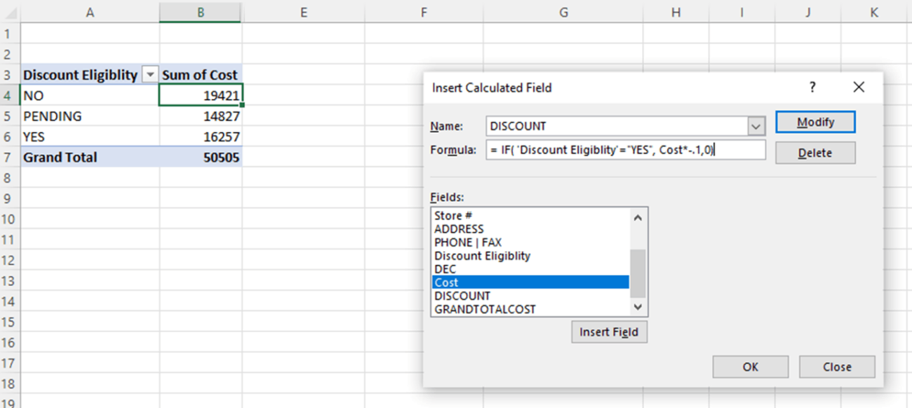
1. Create a Calculated Field or Item
Calculated fields and items allow you to perform custom calculations within your PivotTable without altering the source data.
- Calculated Field: Add a new column by creating formulas that apply across the entire dataset. For example, calculate profit by subtracting costs from revenue.
- Calculated Item: Perform calculations within a specific field, such as finding the percentage difference between two categories.
How to Create:
- Click inside the PivotTable.
- Go to the “PivotTable Analyze” tab (or “Options” in older versions).
- Select “Fields, Items & Sets” and choose “Calculated Field” or “Calculated Item.”
2. Use the Grouping Feature
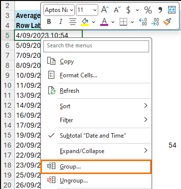
Grouping allows you to organize data into meaningful categories, such as:
- Date Grouping: Group sales data by months, quarters, or years.
- Number Grouping: Categorize numerical data into ranges, such as ages or income levels.
- Custom Grouping: Combine specific items, such as regions or products, into broader categories.
How to Group:
- Right-click on a field in the PivotTable.
- Select “Group.”
- Choose your desired grouping criteria.
3. Show Values As
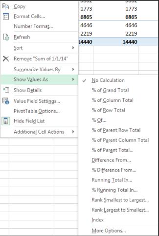
The “Show Values As” feature transforms raw data into meaningful insights by displaying it as percentages, rankings, or differences.
- Percentage of Total: View each item as a percentage of the overall total.
- Rank: Rank items within a category or overall dataset.
- Difference From: Show how values differ from a baseline.
How to Apply:
- Click on a value field in your PivotTable.
- Choose “Show Values As” from the “Value Field Settings” menu.
- Select your desired calculation method.
4. Use Slicers for Dynamic Filtering
Slicers provide an intuitive way to filter data visually, making it easier to explore your dataset.
- Add slicers for fields like product categories, regions, or dates.
- Connect multiple PivotTables to a single slicer for synchronized filtering.
How to Add a Slicer:
- Click on your PivotTable.
- Go to the “PivotTable Analyze” tab.
- Select “Insert Slicer” and choose the field you want to filter by.
5. Create a PivotChart
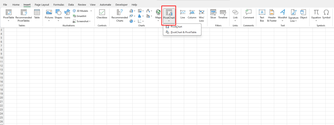
PivotCharts transform your summarized data into visual representations, making it easier to spot trends and patterns.
- Pair a PivotChart with a PivotTable for an interactive dashboard.
- Use slicers and filters to dynamically update your chart.
- Experiment with different chart types, such as bar, line, or pie charts.
How to Create:
- Select your PivotTable.
- Go to the “Insert” tab.
- Choose a chart type under the “Charts” section.
6. Filter with the Value Filters Feature
Value Filters help you focus on the most critical data points by filtering based on numerical conditions.
- Top 10 Filter: Highlight the top-performing products or regions.
- Greater Than Filter: Show only values exceeding a specific threshold.
- Custom Filters: Combine multiple conditions to refine your dataset.
How to Apply:
- Click the dropdown arrow next to a field in the PivotTable.
- Choose “Value Filters” and define your criteria.
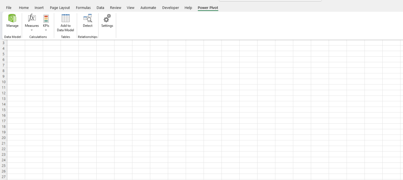
7. Use Power Pivot for Complex Data Models
Power Pivot extends the capabilities of standard PivotTables by enabling you to work with large datasets and create relationships between multiple tables.
- Data Modeling: Combine data from different sources without merging them.
- DAX Formulas: Use Data Analysis Expressions (DAX) to create advanced calculations.
- Memory Efficiency: Handle millions of rows without performance issues.
How to Enable Power Pivot:
- Go to “File” > “Options” > “Add-ins.”
- Select “COM Add-ins” and enable “Microsoft Power Pivot for Excel.”
8. Refresh Data Automatically
Keeping your PivotTable up-to-date is essential for accurate analysis.
- Set your PivotTable to refresh automatically when you open the workbook.
- Use the “Refresh All” button to update multiple PivotTables simultaneously.
How to Automate Refreshing:
- Right-click on your PivotTable.
- Choose “PivotTable Options.”
- Under the “Data” tab, check “Refresh data when opening the file.”
9. Drill Down for Detailed Data
Drill-down functionality allows you to quickly view the raw data behind a summarized value.
- Double-click on any cell in the PivotTable to generate a new sheet with detailed data for that cell.
- Use this feature to investigate anomalies or explore specific data points.
Get the best deals on the cheapest Office keys for your productivity needs.

