How to use INDIRECT for Dynamic Range Referencing?

The INDIRECT function in Excel is a powerful tool that allows you to create dynamic references to cells, ranges, or even sheets. It enables you to change the reference in a formula without manually editing it, which is especially useful for large, complex workbooks.

Here’s a step-by-step guide on how to use the INDIRECT function for dynamic range referencing.

Step 1: Understand the Basics of INDIRECT

The INDIRECT function takes a text string and converts it into a valid cell or range reference. Its syntax is simple:

=INDIRECT(ref_text, [a1])

• ref_text: This is the reference in text form that you want to convert into an actual reference.
• a1: An optional argument that specifies whether the reference is in A1 or R1C1 style. It defaults to TRUE (A1 style).

Step 2: Create a Simple Example

To understand how INDIRECT works, let’s start with a simple example. Assume you have the following values:

• In A1: “SalesData”
• In B1: 100

We’ll use INDIRECT to reference the content of A1 and return the value from the named range SalesData.

1. In A2, enter the formula:

=INDIRECT("B1")

2. The result will be 100, as INDIRECT converts the text “B1” into the actual cell reference.

Step 3: Create Dynamic Range References

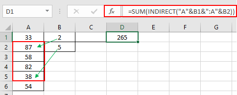
Now let’s apply INDIRECT to create a dynamic range reference that changes based on user input or other conditions.

1. Assume you have a data set in Sheet1, ranging from A1and B1.
2. In C1, allow the user to input either “A” or “B”.
3. Use the following formula to reference column A or B dynamically based on the input in C1:

=SUM(INDIRECT("Sheet1!" & C1 & "1:" & C1 & "10"))

This formula dynamically refers to either A1 or B1 depending on whether the user enters “A” or “B” in C1.

How to Use INDIRECT for Dynamic Range Referencing in Excel: A Step-by-Step Guide

The INDIRECT function in Excel is a powerful tool that allows you to create dynamic references to cells, ranges, or even sheets. It enables you to change the reference in a formula without manually editing it, which is especially useful for large, complex workbooks. Here’s a step-by-step guide on how to use the INDIRECT function for dynamic range referencing.

Step 1: Understand the Basics of INDIRECT

The INDIRECT function takes a text string and converts it into a valid cell or range reference. Its syntax is simple:

=INDIRECT(ref_text, [a1])

• ref_text: This is the reference in text form that you want to convert into an actual reference.
• a1: An optional argument that specifies whether the reference is in A1 or R1C1 style. It defaults to TRUE (A1 style).

Step 2: Create a Simple Example

To understand how INDIRECT works, let’s start with a simple example. Assume you have the following values:

• In A1: “SalesData”
• In B1: 100

We’ll use INDIRECT to reference the content of A1 and return the value from the named range SalesData.

1. In A2, enter the formula:scssCopy code=INDIRECT("B1")
2. The result will be 100, as INDIRECT converts the text “B1” into the actual cell reference.

Step 3: Create Dynamic Range References

Now let’s apply INDIRECT to create a dynamic range reference that changes based on user input or other conditions.

1. Assume you have a data set in Sheet1, ranging from A1and B1.
2. In C1, allow the user to input either “A” or “B”.
3. Use the following formula to reference column A or B dynamically based on the input in C1:lessCopy code=SUM(INDIRECT("Sheet1!" & C1 & "1:" & C1 & "10")) This formula dynamically refers to either A1or B1depending on whether the user enters “A” or “B” in C1.

Step 4: Use INDIRECT with Named Ranges

You can also use INDIRECT to reference named ranges dynamically. This is useful when you have multiple named ranges and want to switch between them without hard-coding the references.

1. Create two named ranges, Q1Sales for A1and Q2Sales for B1.
2. In C1, let the user choose either “Q1Sales” or “Q2Sales”.
3. Use the following formula to dynamically reference the named range:

=SUM(INDIRECT(C1))

If the user enters “Q1Sales” in C1, the formula will sum the values from A1. If they enter “Q2Sales”, it will sum B1

Step 5: Use INDIRECT with Multiple Sheets

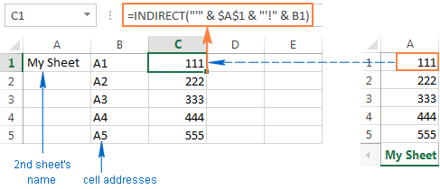
INDIRECT can also reference data across different sheets. This is particularly useful for workbooks with similar structures across multiple sheets.

1. Assume you have data in Sheet1 and Sheet2, both with values in A1.
2. In B1, allow the user to enter either “Sheet1” or “Sheet2”.
3. Use the following formula to dynamically reference the data in the chosen sheet:

=SUM(INDIRECT(B1 & "!A1:A5"))

This formula sums the values in A1 of the sheet specified in B1.

Step 6: Apply INDIRECT with Data Validation

You can combine INDIRECT with data validation to make selections more dynamic and user-friendly.

1. In C1, create a data validation list allowing users to choose between “Q1Sales” and “Q2Sales”.
2. In D1, use the formula:

=SUM(INDIRECT(C1))

This lets users select from a dropdown, and the sum will dynamically update based on their choice.

Step 7: Combine INDIRECT with Other Functions

INDIRECT can be combined with other Excel functions like VLOOKUP, INDEX, and MATCH to make your formulas even more dynamic.

For example, you can combine INDIRECT with VLOOKUP to look up data from different sheets dynamically.

1. In B1, enter the name of the sheet (e.g., “SalesData”).
2. Use the following formula to perform a VLOOKUP on the specified sheet:

=VLOOKUP(A2, INDIRECT("'" & B1 & "'!A2:B10"), 2, FALSE)

This allows you to look up data from the sheet specified in B1.

Get genuine Office Keys at the lowest prices available!