How can I Protect Specific Cells while llowing edits to others in Excel?

In Excel, there are times when you may want to protect certain cells from being edited while allowing others to be modified. This feature is useful for securing important data while letting users input or update other parts of the worksheet. Here’s a step-by-step guide to help you protect specific cells while leaving others editable in Excel.

Step 1: Select All Cells to Unlock by Default

By default, Excel locks all cells when you protect the sheet. The first step is to unlock the cells you want to allow edits on.

1. Select the entire worksheet by clicking the small triangle at the top-left corner between row 1 and column A (or press Ctrl + A).
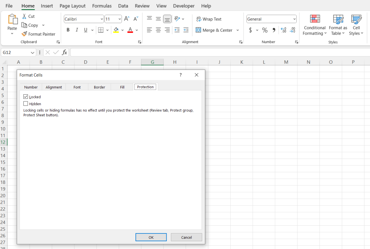
2. Right-click on the selection and choose Format Cells.
3. In the Format Cells window, go to the Protection tab.
4. Uncheck the box next to Locked and click OK.

Now, all cells in the worksheet are unlocked, meaning they can be edited once you protect the sheet.

Step 2: Lock the Cells You Want to Protect

Next, select the specific cells that you want to protect from editing.

1. Highlight the cells you want to protect (e.g., headers, formulas, or key data).
2. Right-click on the selected cells and choose Format Cells.
3. In the Protection tab, check the box next to Locked and click OK.

These cells will now be locked once the sheet is protected, preventing any edits to them.

Step 3: Protect the Worksheet

To enforce the protection, you need to protect the entire worksheet.

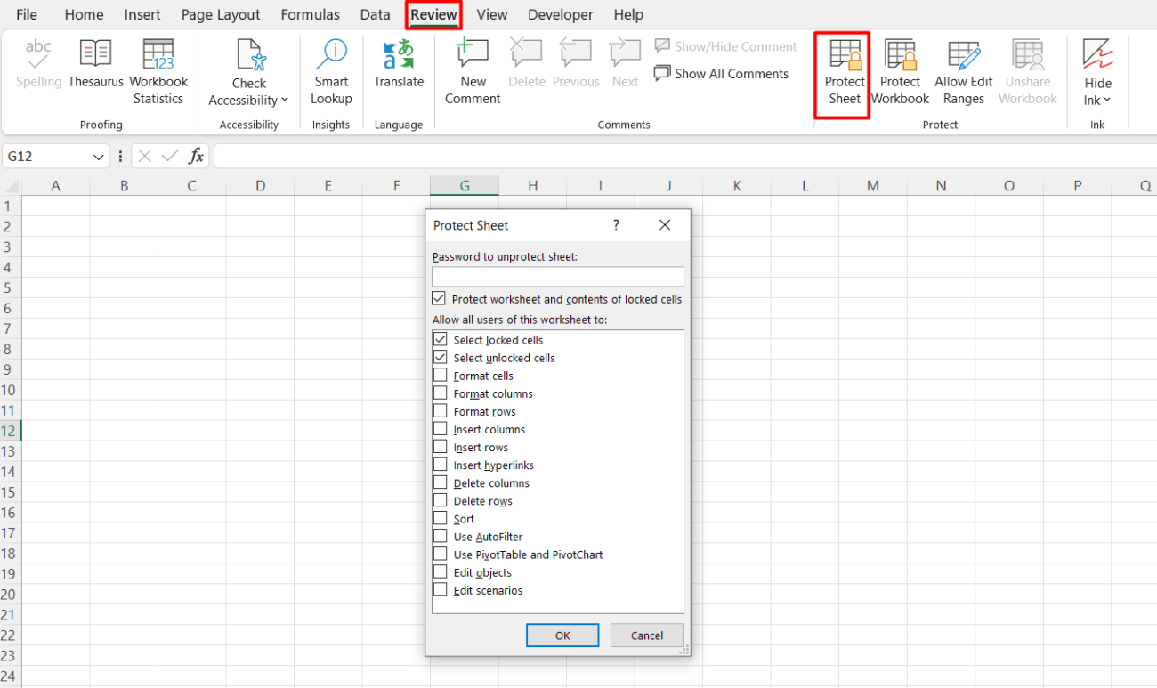
1. Go to the Review tab on the ribbon.
2. Click Protect Sheet.
3. In the Protect Sheet dialog box, you can set a password to prevent others from unprotecting the sheet (optional, but recommended for security).
4. Make sure the option Protect worksheet and contents of locked cells is selected.
5. You can also specify which actions users are allowed to perform on the sheet, such as selecting locked or unlocked cells.
6. Click OK.

Now, the specific cells you locked are protected, while the rest of the worksheet remains editable.

Step 4: Test the Protection

To ensure everything is set up correctly, try editing different parts of the sheet.

1. Attempt to edit one of the locked cells—you should see an error message indicating the cell is protected.
2. Try editing the unlocked cells—these should be editable without any issues.

Step 5: Unprotect the Sheet (If Needed)

If you ever need to make changes to the locked cells or modify the protection settings:

1. Go to the Review tab.
2. Click Unprotect Sheet.
3. Enter the password if one was set.
4. Now, you can make any necessary changes and protect the sheet again by following the same steps.

Step 6: Optional: Allow Specific Users to Edit Certain Cells

Excel also provides the option to allow specific users to edit certain locked cells while keeping the rest of the sheet protected.

1. Go to the Review tab and click Allow Users to Edit Ranges.
2. In the dialog box, define ranges and assign permissions for specific users (this feature requires a network setup and may not be available in all versions of Excel).
3. After setting permissions, protect the sheet as usual.

Step 7: Save Your Protected Workbook

Once you’ve set up cell protection, save your workbook to keep these settings in place.

1. Click File and select Save or Save As to save your protected worksheet.

Get genuine Office Keys at the lowest prices available on our website for unbeatable savings and instant access.