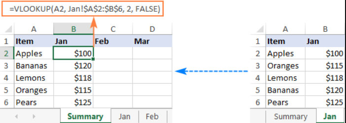
How can I use VLOOKUP across Multiple Sheets in Excel?

The VLOOKUP function in Excel allows you to search for and retrieve data from a specific table or range. While it’s typically used within a single sheet, you can also use VLOOKUP to pull data from different sheets in the same workbook. This guide will walk you through using VLOOKUP across multiple sheets in Excel.

Step 1: Organize Your Data

Ensure your data is properly structured across multiple sheets. For example:

• In Sheet1, you might have a list of employee IDs.
• In Sheet2, you could have more detailed employee data, such as names and departments.

The goal is to pull data (e.g., names) from Sheet2 into Sheet1 using the employee IDs.

Step 2: Start Writing the VLOOKUP Formula

In the sheet where you want to display the retrieved data (e.g., Sheet1), follow these steps:

1. Click on the cell where you want the result to appear.
2. Start writing the VLOOKUP formula by entering the function name and opening parentheses.

Step 3: Select the Lookup Value

The first piece of information in the VLOOKUP formula is the lookup value, which is the value you want to search for in the other sheet. In this case, it will be the employee ID from Sheet1.

1. Click on the cell that contains the employee ID you want to search for.

Step 4: Specify the Table Array in the Other Sheet

Next, you need to tell Excel where to look for the data. This range of data (the table array) is located in Sheet2.

1. Switch to Sheet2.
2. Select the range of cells that includes both the employee IDs and the data you want to retrieve, such as names.

Excel will now know to look for the employee IDs in Sheet2.

Step 5: Specify the Column Index Number

The column index number tells Excel which column in your data range contains the information you want to retrieve. For instance, if names are in the second column of your selected data range, you would use column number 2.

1. Identify the correct column number where the desired data is located (e.g., the second column for names).

Step 6: Choose an Exact Match

In most cases, you will want an exact match for the value you’re looking up. To do this, select the option for an exact match in the VLOOKUP function.

1. Indicate that you want Excel to return only exact matches for the lookup value.

Step 7: Copy the Formula to Other Cells

Once you’ve created the VLOOKUP formula, you can copy it down to other cells to apply it to the entire list of employee IDs.

1. Click on the cell with the VLOOKUP formula.
2. Drag the formula down to apply it to other rows. This allows you to retrieve data for each employee automatically.

Get genuine Office Keys at the lowest prices available on our website for unbeatable savings and instant access.