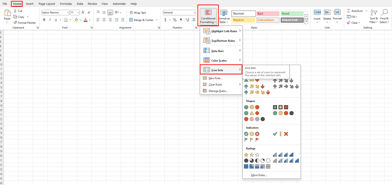
How can you Conditional Format using Icons in Excel?

Conditional formatting in Excel is a fantastic tool for visualizing data and quickly understanding trends and patterns. One powerful feature within conditional formatting is the use of icons to provide visual cues. In this blog post, we’ll walk you through the step-by-step process of using conditional formatting with icons in Excel.

Step 1: Open Your Excel Workbook

1. Launch Microsoft Excel.
2. Open the workbook that contains the data you want to format.

Step 2: Select the Range of Cells

1. Click on the top-left cell of the range you want to apply conditional formatting to.
2. Drag the cursor to cover the entire range, or use keyboard shortcuts:
   • Press Ctrl + A to select the entire worksheet.
   • Hold down Shift and press the arrow keys to select a custom range.

Step 3: Access Conditional Formatting

1. Go to the Home tab on the ribbon.
2. Click on Conditional Formatting in the Styles group.
3. A dropdown menu will appear with various conditional formatting options.

Step 4: Choose an Icon Set

1. From the dropdown menu, hover over Icon Sets.
2. Select the type of icon set you want to use. Options include arrows, shapes, flags, and more.

Step 5: Customize the Icon Set Rule

1. After selecting an icon set, a default rule will be applied to your range.
2. To customize this rule, go back to Conditional Formatting in the Home tab.
3. Select Manage Rules at the bottom of the dropdown menu.
4. In the Conditional Formatting Rules Manager, select the rule you want to edit and click Edit Rule.

Step 6: Configure Icon Set Options

1. In the Edit Formatting Rule dialog box, under the Edit the Rule Description section, you can configure how the icons are assigned based on cell values.
2. Choose between different criteria such as percentage, percentile, number, or formula.
3. Specify the value thresholds for each icon. Adjust the default values as needed to suit your dataset.

Step 7: Apply and Save the Rule

1. After setting up the rule criteria, click OK to save your custom rule.
2. In the Conditional Formatting Rules Manager, click Apply to implement the changes.
3. Click OK to close the manager.

Final Step: Save Your Workbook

1. Click on File.
2. Select Save or Save As to save your workbook with the newly applied conditional formatting.

Unlock the full potential of your productivity by purchasing the cheapest Office Keys available, offering all the features you need at an unbeatable price.