How do I use Conditional Formatting to Highlight Duplicate Values in Excel?

Conditional formatting in Excel is a powerful tool that allows you to automatically apply formatting to cells based on specific conditions. One of the most common uses of this feature is to highlight duplicate values in a dataset. This guide will walk you through the steps to easily highlight duplicate values using conditional formatting in Excel.

Step 1: Select the Data Range

First, decide which range of data you want to check for duplicates.

1. Click and drag to select the cells where you want to apply conditional formatting.
   • For example, if you want to highlight duplicate values in column A, select the entire column, or highlight specific rows if the range is smaller.

Step 2: Open the Conditional Formatting Menu

After selecting the data range, access the conditional formatting options.

1. Go to the Home tab in the Excel ribbon.
2. In the Styles group, click on Conditional Formatting.
3. From the dropdown menu, select Highlight Cells Rules, and then choose Duplicate Values.

Step 3: Set the Duplicate Highlighting Rule

Once you’ve selected Duplicate Values, a dialog box will appear.

1. In the dialog box, you’ll see two options: one for highlighting Duplicate or Unique values, and another for choosing the format.
2. Make sure Duplicate is selected.
3. From the second dropdown, choose the formatting style you prefer. By default, Excel uses light red fill with dark red text, but you can customize this to suit your needs.

Step 4: Apply the Conditional Formatting

After choosing the formatting style, click OK to apply the rule.

1. Excel will automatically highlight any duplicate values within the selected range based on the formatting you chose.

Step 5: Customize or Edit the Rule (Optional)

If you need to adjust the formatting rule, you can easily modify it:

1. Go back to the Home tab and click Conditional Formatting.
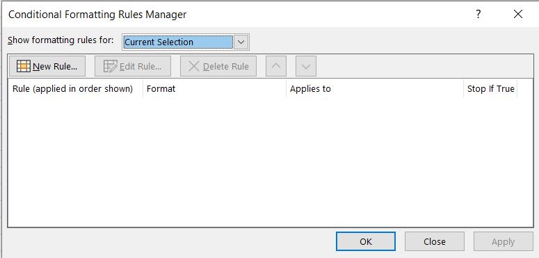
2. Select Manage Rules from the dropdown menu.
3. In the Conditional Formatting Rules Manager window, you can edit, delete, or create new rules.

Step 6: Expand or Narrow the Range (Optional)

If you need to apply the duplicate formatting to a larger or smaller range after creating the rule:

1. Select the new data range.
2. Repeat the conditional formatting process by either editing the existing rule or applying the duplicate values rule to the new selection.

Step 7: Remove Conditional Formatting (If Needed)

If you decide that you no longer need the duplicate highlighting:

1. Go to the Home tab, click Conditional Formatting, and choose Clear Rules.
2. You can clear rules for the selected cells or the entire sheet, depending on your needs.

Get genuine Office Keys at the lowest prices available on our website for unbeatable savings and instant access.