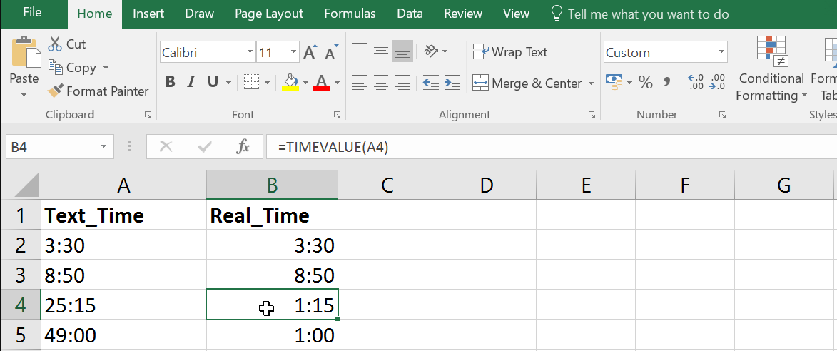
How to use the TIMEVALUE Function in Excel?

The TIMEVALUE function in Excel is a powerful tool that allows you to convert text representations of time into actual Excel time values. This is particularly useful for performing time-based calculations, formatting, and sorting. Follow this step-by-step guide to master the TIMEVALUE function.

Step 1: Open Your Excel File

1. Launch Excel: Start Microsoft Excel on your computer.
2. Open an Existing Workbook: Go to “File” > “Open” and browse for the workbook containing the text times you want to convert. Double-click to open it.
3. Select the Appropriate Worksheet: Navigate to the worksheet that includes the text times.

Step 2: Identify the Text Times

1. Locate Text Times: Identify the cells that contain the text representations of time. These will usually be in a column.
2. Format Check: Ensure that the text times are in a format that the TIMEVALUE function can interpret (e.g., “HH:MM:SS AM/PM” or “HH:MM”).

Step 3: Select the Destination Cell for the TIMEVALUE Function

1. Choose Target Cell: Click on the cell where you want the resultant Excel time to appear (e.g., if your text time is in cell A1, you might use cell B1 for the TIMEVALUE function).

Step 4: Enter the TIMEVALUE Function

1. Activate Formula Mode: In your target cell, start by typing an equals sign = to enter formula mode.
2. Type TIMEVALUE: Begin typing TIMEVALUE( to initiate the function.
3. Add Cell Reference: Click on the cell with the text time (e.g., A4) to add it to the formula, or manually type A4.
4. Close Parenthesis: Type ) to close the function and complete the formula. Your formula should look like this: =TIMEVALUE(A4)
5. Press Enter: Hit Enter on your keyboard to execute the function.

Step 5: Copy the Formula to Adjacent Cells (If Needed)

1. Select the Formula Cell: Click on the cell with the TIMEVALUE function (e.g., B1).
2. Drag the Fill Handle: Hover over the bottom-right corner of the cell until you see a small ‘+’ sign. Click and drag down or across to copy the formula to adjacent cells.
3. Release Mouse Button: Release the mouse button when you have covered all the necessary cells. Excel will auto-update the formulas to reference the corresponding text time cells.

Step 6: Convert Resulting Numbers to Time Format

1. Select Resultant Times: Highlight the cells containing the TIMEVALUE results.
2. Open Format Cells Dialogue: Right-click and choose “Format Cells” from the context menu, or press Ctrl + 1.
3. Choose Time Format: In the “Format Cells” dialogue box, go to the “Number” tab. Select “Time” from the Category list.
4. Pick Time Type: Choose the desired time format from the available options.
5. Apply Format: Click “OK” to apply the time format.

Step 7: Adjust Any Necessary Formatting

1. Check Columns: Ensure that columns are wide enough to display the new time values correctly. Adjust column width if necessary.
2. Apply Additional Formatting: Apply any additional formatting styles (font size, color, bold, borders, etc.) to match your workbook’s design.

Step 8: Save Your Workbook

1. Save Your Work: Click on “File” > “Save” or press Ctrl + S to save the existing workbook.
2. Save As New Version: If you want to preserve the original data, select “File” > “Save As” and create a new version of your workbook.

Get genuine Office Keys at unbeatable prices on our website – your ultimate destination for affordable software solutions!