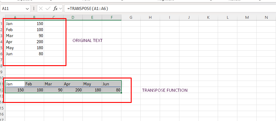
How to use the TRANSPOSE Function in Excel?

The TRANSPOSE function in Excel allows you to switch the orientation of your data, converting rows to columns and columns to rows. This can be useful when you have a large amount of data that needs to be organized in a different way. Follow these detailed steps to use the TRANSPOSE function effectively.

Step 1: Open Your Excel File

1. Launch Excel: Open Microsoft Excel on your computer.
2. Open Existing Workbook: Navigate to “File” > “Open” and locate the workbook that contains the data you want to transpose. Double-click the file to open it.
3. Select Worksheet: Make sure you are on the worksheet that contains the data you wish to transpose.

Step 2: Select and Copy the Data

1. Highlight the Data: Click and drag your mouse to select the range of data you want to transpose.
2. Copy the Data: Right-click the selected range and choose “Copy,” or press Ctrl + C on your keyboard.

Step 3: Choose Destination for Transposed Data

1. Select New Location: Click on the cell where you want your transposed data to start (this will be the top-left corner of the new range). This cell should not overlap with the existing data range.
2. Ensure Enough Space: Make sure there are enough blank rows and columns to accommodate the transposed data.

Step 4: Enter the TRANSPOSE Function

1. Enter Formula Mode: With the target cell selected, enter formula mode by typing an equals sign =.
2. Type TRANSPOSE: Start typing TRANSPOSE( to trigger the function. Excel will prompt you with the function name.
3. Highlight Original Data: Inside the parentheses, click and drag to reselect the original data range or manually enter the range address (e.g., A1:D4).
4. Close Parenthesis: Type a closing parenthesis ) to complete the function and press Enter.

Step 5: Complete the Transpose Operation (Array Formula for Old Versions)

1. Activate Array Formula: For older versions of Excel (before Excel 365), you need to enter this as an array formula by pressing Ctrl + Shift + Enter. If your version automatically supports dynamic arrays, just pressing Enter will suffice.

Step 6: Adjust Any Formatting as Needed

1. Apply Cell Formatting: If needed, apply any formatting to your newly transposed data to match the original format. You can change font styles, colors, borders, and more, using the options under the “Home” tab.
2. Check References: Double-check any formulas or references in your transposed data to ensure they are still accurate.

Step 7: Save Your Workbook

1. Save Progress: Save your changes by clicking “File” > “Save” or pressing Ctrl + S.
2. Save As New Version: If you wish to keep the original data unchanged, click “File” > “Save As” and create a new version of the workbook.

Unlock the full potential of your productivity suite with our genuine Office Keys, now available at unbeatable low prices!