
5 Excel Functions Every Professional Should Know
Microsoft Excel is a cornerstone tool for data analysis, budgeting, project management, and so much more. But, to get the most out of Excel, it’s essential to know key functions that can simplify tasks, save time, and improve accuracy. Here are five Excel functions every professional should know to boost productivity and make the most of their data.
1. VLOOKUP: Streamline Data Searches
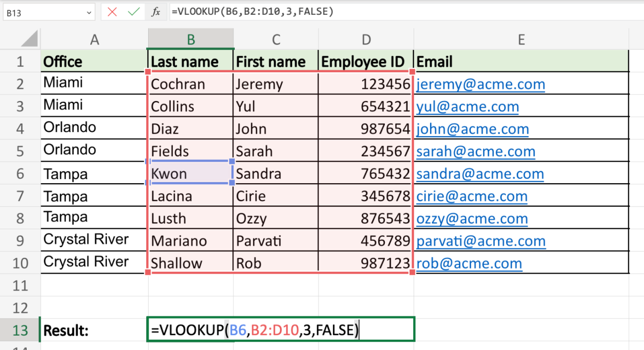
The VLOOKUP function is one of Excel’s most popular functions for looking up specific information in large datasets. It’s a lifesaver when you need to find related data across different tables or sheets.
- Formula:
=VLOOKUP(lookup_value, table_array, col_index_num, [range_lookup]) - Example: Say you have a table with product IDs in column A and prices in column B. To find the price of a specific product, use
=VLOOKUP("ProductID", A2:B10, 2, FALSE).
Key Points:
- lookup_value: The value you’re searching for.
- table_array: The range of cells that contains the data.
- col_index_num: The column number in the range where the result is located.
- range_lookup: Use
FALSEfor an exact match,TRUEfor an approximate match.
With VLOOKUP, you can easily pull related data from large datasets, saving you the hassle of manually searching rows and columns.
2. IF: Make Decisions with Conditions
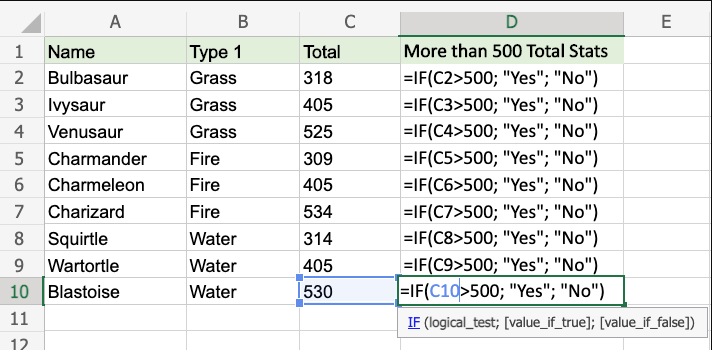
The IF function allows you to perform logical tests and return specific values based on whether the result is true or false. This is especially helpful when you need to categorize data or apply different calculations based on criteria.
- Formula:
=IF(logical_test, value_if_true, value_if_false) - Example: For instance, to display “Pass” if a student score in A2 is 50 or above, otherwise “Fail”, use
=IF(A2 >= 50, "Pass", "Fail").
Key Points:
- logical_test: The condition you’re evaluating (e.g., A2 >= 50).
- value_if_true: The result if the condition is met.
- value_if_false: The result if the condition isn’t met.
Using IF statements helps to classify data, create flags, or automate decision-making processes in your spreadsheets.
3. SUMIF: Sum Values Based on Criteria
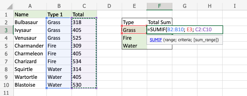
The SUMIF function combines the functionality of the SUM function with a conditional filter. This function is perfect for situations where you only want to sum data that meets certain criteria.
- Formula:
=SUMIF(range, criteria, [sum_range]) - Example: To calculate total sales for “Product A” in column B, with sales data in column C, you’d use
=SUMIF(B2:B20, "Product A", C2:C20).
Key Points:
- range: The range of cells that you want to apply criteria to.
- criteria: The condition the data must meet.
- sum_range: The cells you want to sum (if different from the range).
SUMIF helps you quickly analyze totals for specific items, regions, time periods, or any category you need to filter by.
4. CONCATENATE (or CONCAT): Combine Text from Multiple Cells
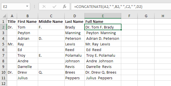
The CONCATENATE (or simply CONCAT) function allows you to combine text from multiple cells into one cell, which is useful for creating full names, generating product codes, or formatting addresses.
- Formula:
=CONCATENATE(text1, [text2], ...)or=CONCAT(text1, text2, ...) - Example: To combine a first name in cell A2 and a last name in cell B2, use
=CONCATENATE(A2, " ", B2).
Key Points:
- text1, text2: The text items or cell references you want to combine.
- You can also use “&” as a shortcut, like
=A2 & " " & B2.
This function is valuable for organizing data and creating labels, codes, or unique identifiers without manually combining cell values.
5. INDEX and MATCH: A More Powerful Alternative to VLOOKUP
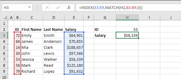
While VLOOKUP is great, INDEX and MATCH are a powerful duo for data retrieval, offering more flexibility and accuracy. Unlike VLOOKUP, which only works left-to-right, INDEX and MATCH can retrieve data from any direction and work faster with large datasets.
- Formula:
=INDEX(return_range, MATCH(lookup_value, lookup_range, [match_type])) - Example: To find the price of a product with ID “P123” in a table where IDs are in column B and prices are in column A, use
=INDEX(A2:A10, MATCH("P123", B2:B10, 0)).
Key Points:
- INDEX: Returns the value in a specified cell range based on row and column numbers.
- MATCH: Returns the relative position of an item within a range.
Using INDEX and MATCH, you get greater flexibility in data lookup and retrieval than with VLOOKUP, especially in complex tables.
Get genuine Microsoft Office keys at affordable prices and enjoy premium productivity tools without breaking the bank!

