Mastering Excel Formulas: Tips for Beginners
Excel formulas are the backbone of Excel’s powerful data analysis capabilities, allowing you to automate calculations, analyze data, and organize information with ease. For beginners, diving into formulas can seem intimidating, but mastering the basics will make you more efficient and open up Excel’s full potential. Here’s a guide to help you get started with essential Excel formulas and helpful tips for mastering them.
1. Understand Excel’s Formula Basics
Before jumping into complex formulas, it’s helpful to understand how Excel formulas work. Here are the basics:
- All formulas start with an equal sign (
=), letting Excel know you’re entering a calculation. - Formulas can include operators like
+(addition),-(subtraction),*(multiplication), and/(division). - Cell references (like
A1orB2) allow you to pull in data from other cells. This is key because it means your calculations can update automatically if the values in those cells change.
2. Start with Simple Functions
Excel has a variety of built-in functions that make calculations easier. Let’s look at a few essential ones:
- SUM: Adds up numbers in a range. Use
=SUM(A1:A10)to total up values from cells A1 to A10. - AVERAGE: Calculates the mean of values in a range.
=AVERAGE(B1:B10)finds the average value in that range. - COUNT: Counts the number of cells in a range that contain numbers. Use
=COUNT(C1:C10)to get the count of numeric cells in C1 to C10.
These functions are straightforward yet powerful. Practice using them with different ranges to become comfortable with basic calculations.
3. Use AutoSum for Quick Calculations
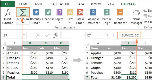
One of the quickest ways to add up a range of numbers is by using the AutoSum feature. Simply select the cell where you want the result to appear, go to the Home tab, and click on AutoSum (∑). Excel will automatically select the most likely range to sum, and you can adjust the range if necessary before pressing Enter.

4. Master Cell Referencing: Relative, Absolute, and Mixed
Excel offers three types of cell referencing, each useful in different situations:
- Relative referencing (like
A1) changes based on the position when you copy the formula to another cell. - Absolute referencing (like
$A$1) keeps the cell reference fixed, even if the formula is moved or copied. - Mixed referencing (like
$A1orA$1) keeps either the column or row constant while allowing the other to change.
Learning how to use these references will help you work more efficiently with formulas, especially in larger spreadsheets. To change a reference type, simply add the $ symbol in front of the row or column you want to lock.
5. Learn Logical Formulas with IF
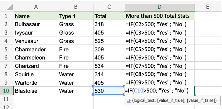
The IF function is one of the most useful tools in Excel, allowing you to make decisions based on a condition.
- Formula:
=IF(condition, value_if_true, value_if_false) - Example: If you want to check if a cell (A2) has a value greater than 50, use
=IF(A2 > 50, "Pass", "Fail").
This formula will display “Pass” if the condition is met and “Fail” if not. The IF function is a great way to add automation to your spreadsheets, and it becomes even more powerful when combined with other functions.

6. Utilize the Fill Handle for Formula Replication
The Fill Handle (a small square at the bottom-right corner of a selected cell) is an easy way to copy a formula across a range. Simply drag the fill handle down or across, and Excel will copy the formula to each cell, automatically adjusting cell references. This feature saves you time and helps apply formulas consistently across multiple rows or columns.
7. Combine Text with CONCATENATE (or CONCAT)
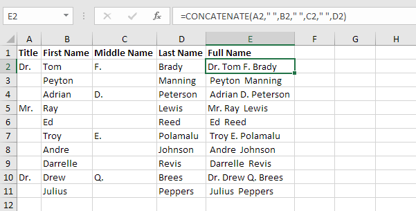
Combining text from different cells is helpful for creating labels, product codes, or full names from separate first and last name columns. Use the CONCATENATE or CONCAT function to join cells:
- Formula:
=CONCATENATE(cell1, cell2, ...)or=CONCAT(cell1, cell2, ...) - Example: To combine a first name in A2 with a last name in B2, use
=CONCAT(A2, " ", B2).
This formula makes it easy to organize and display data in a readable format.

8. Get Comfortable with Error Handling Using IFERROR
As you start working with more formulas, you may encounter errors, such as #DIV/0! when dividing by zero or #VALUE! when using incompatible data types. The IFERROR function can help you handle these gracefully.
- Formula:
=IFERROR(formula, value_if_error) - Example: If you have a division formula
=A2/B2, you can use=IFERROR(A2/B2, "Error")to display “Error” instead of an error message.
Using IFERROR keeps your spreadsheets clean and user-friendly, especially if others will view or interact with them.
9. Explore Excel’s Formula Help
Excel’s Insert Function feature provides a detailed guide for each function. Select an empty cell, go to the Formulas tab, and click Insert Function. From there, you can search for functions, select one, and get a detailed description of how it works. It’s a handy tool if you’re ever unsure about a formula’s syntax or purpose.
10. Practice and Experiment
The best way to master Excel formulas is to practice. Start with simple exercises, like calculating totals, averages, and percentages. Gradually incorporate more advanced functions like IF, COUNTIF, or VLOOKUP as you get comfortable. Remember, the more you work with formulas, the more intuitive they’ll become.
Get affordable, genuine Office Keys to unlock the full range of Microsoft Office features at a fraction of the usual cost.

