Using Conditional Formatting in Excel to Highlight Key Data
Conditional formatting in Excel is a powerful feature that allows users to visually emphasize important data points within a spreadsheet. By applying different formatting options based on specific conditions, you can easily identify trends, patterns, and outliers in your data. This guide will explore how to use conditional formatting effectively to highlight key data in Excel.
Why Use Conditional Formatting?
Conditional formatting enhances data visualization and helps users quickly grasp complex information. Here are a few benefits:
- Improved Readability: By highlighting critical data, you make your spreadsheet more accessible.
- Quick Analysis: It allows for fast identification of trends, anomalies, or specific criteria without extensive manual review.
- Customization: You can tailor the formatting rules to suit your specific needs, making your data analysis more relevant.
Getting Started with Conditional Formatting
- Open Your Excel Workbook: Launch Excel and open the workbook containing the data you want to analyze.
- Select Your Data Range: Click and drag to highlight the cells you wish to format based on specific criteria.
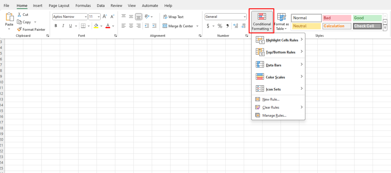
- Navigate to Conditional Formatting:
- Go to the Home tab on the Ribbon.
- Click on Conditional Formatting in the Styles group. You will see several options for applying formatting rules.

Types of Conditional Formatting
1. Highlight Cell Rules
This option allows you to format cells based on their values. Here are some common rules:
- Greater Than/Less Than: Highlight cells that are greater than, less than, or equal to a specified value.
- Example: To highlight sales figures greater than $1,000:
- Select Highlight Cell Rules > Greater Than.
- Enter
1000and choose a formatting style (e.g., green fill).
- Example: To highlight sales figures greater than $1,000:
- Between: Highlight cells that fall within a specified range.
- Example: To highlight expenses between $200 and $500:
- Select Highlight Cell Rules > Between.
- Enter
200and500and select a format.
- Example: To highlight expenses between $200 and $500:
- Text that Contains: Format cells containing specific text.
- Example: Highlight all cells containing “urgent”:
- Select Text that Contains and enter “urgent.”
- Example: Highlight all cells containing “urgent”:
2. Top/Bottom Rules
Highlight the top or bottom values in your selected range.
- Top 10 Items: Highlight the top 10 highest values in your data set.
- Go to Top/Bottom Rules > Top 10.
- Choose how many items to highlight and select a formatting style.
- Bottom 10%: Highlight the bottom 10% of values in your selection.
- Select Top/Bottom Rules > Bottom 10% and choose your formatting.
3. Data Bars
Data bars provide a visual representation of the value within the cell.
- To add data bars:
- Select Data Bars from the Conditional Formatting menu.
- Choose a color style, and Excel will fill each cell with a bar reflecting the value’s magnitude.
4. Color Scales
Color scales allow you to apply a gradient color format to your data, indicating value ranges.
- To use color scales:
- Click on Color Scales in the Conditional Formatting menu.
- Choose from the available color gradients to show data distribution visually (e.g., a green-to-red scale where green represents high values and red represents low values).
5. Icon Sets
Icon sets allow you to use symbols to represent data visually.
- To add icon sets:
- Select Icon Sets from the Conditional Formatting menu.
- Choose an icon set (e.g., arrows, traffic lights) that fits your data context.
Customizing Conditional Formatting Rules
Once you have applied conditional formatting, you may want to customize the rules further:
- Manage Rules:
- Go to Conditional Formatting > Manage Rules.
- This opens the Conditional Formatting Rules Manager, where you can edit, delete, or change the order of your formatting rules.
- Edit a Rule:
- Select the rule you want to edit, click Edit Rule, and make your changes. For example, you can modify the condition, the format, or the data range it applies to.
- Delete a Rule:
- Select the rule you wish to remove and click Delete Rule.
Get affordable, genuine Office Keys to unlock the full range of Microsoft Office features at a fraction of the usual cost.

