How can I Combine Text from Multiple Cells in Excel?
Combining text from multiple cells in Excel is a useful way to merge data without manually typing everything. Whether you need to merge first and last names, addresses, or other data, Excel offers a few simple ways to do this. Follow this step-by-step guide to easily combine text from multiple cells in Excel.
Step 1: Select the Cell for the Combined Text
Choose the cell where you want the combined text to appear.
- Click on an empty cell where the merged result will be displayed (e.g., in a new column next to your existing data).
Step 2: Use the CONCATENATE or TEXTJOIN Function
Excel provides two functions for combining text: CONCATENATE and TEXTJOIN.
- If you’re using an older version of Excel, use the
CONCATENATEfunction. For example, you can type:- =CONCATENATE(cell1, cell2)
- If you’re using Excel 2016 or later, it’s better to use
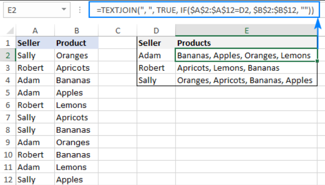
TEXTJOIN, which allows you to add a delimiter like a space or comma between the combined text:- =TEXTJOIN(” “, TRUE, cell1, cell2)

Step 3: Combine Two Cells
To combine text from two cells (e.g., first and last names), use either:
=CONCATENATE(A2, " ", B2)to combine data with a space between, or=TEXTJOIN(" ", TRUE, A2, B2)for the same result in newer versions of Excel.
In this example, if cell A2 has “John” and B2 has “Doe,” the combined result will be “John Doe.”
Step 4: Combine Text from Multiple Cells
If you need to combine text from more than two cells (e.g., for full addresses), simply add more cell references in your formula.
- For
TEXTJOIN, you can include several cells and delimiters. For example:- =TEXTJOIN(“, “, TRUE, A2, B2, C2)
- This combines the data from A2, B2, and C2 with a comma and space between each piece of text.
Step 5: Use Ampersands (&) to Combine Text
An alternative to functions is using the ampersand symbol (&), which also joins text. This method is useful for quick combinations.
- Type
=A2 & " " & B2to combine cells A2 and B2 with a space in between. - You can continue to add more cells and separators as needed.
Step 6: Copy the Formula to Other Rows
Once you’ve created the formula for one row, you can easily apply it to others.
- Click on the cell with the formula.
- Drag the fill handle (the small square at the bottom-right corner of the cell) down to apply the formula to other rows.
Step 7: Convert Formulas to Values (Optional)
If you want to keep the combined text but remove the formula, you can convert the formula results to static values:
- Copy the cells with the formulas.
- Right-click on the selected cells and choose Paste Special.
- Select Values and click OK. This will replace the formula with the actual combined text.
Get Microsoft Office at the lowest price available and enhance your productivity with premium tools.

