How can I use the VLOOKUP Function in Excel?
The VLOOKUP function in Excel is a powerful tool that allows you to quickly find and retrieve data from a large dataset based on a specific criteria. Whether you need to search for information in a table, match values across different worksheets, or perform complex data analysis, understanding how to use the VLOOKUP function can greatly simplify your tasks. This guide will provide a step-by-step walkthrough on how to use the VLOOKUP function in Excel, empowering you to efficiently locate and retrieve data in your spreadsheets.
Excel’s VLOOKUP function offers a versatile solution for searching and retrieving data. We will explore the function’s syntax, including the lookup value, table array, column index, and range lookup parameters. Our guide will cover the process of setting up the function, selecting the appropriate table and columns, and determining the desired output based on the specified criteria. Additionally, we will discuss common challenges and limitations of VLOOKUP, as well as tips and tricks to optimize its use. By following our guide, you will gain a comprehensive understanding of how to effectively utilize the VLOOKUP function in Excel, enabling you to streamline your data analysis tasks and save valuable time and effort.
Step 1: Open Your Excel Workbook
Open the Excel workbook that contains the data you want to work with. If you don’t have a workbook yet, create a new one or use a sample dataset to practice.
Step 2: Select a Cell to Enter the Formula
Choose a cell where you want the VLOOKUP formula results to appear.
Step 3: Enter the VLOOKUP Formula
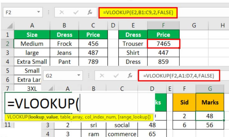
In the selected cell, type the formula “=VLOOKUP(lookup_value, table_array, col_index_num, range_lookup)“. Now, let’s break down each part of the formula:
- lookup_value: This is the value that you want to look up in the table or range.
- table_array: This is the range of cells that contains the table or data range where you want to search for the lookup value.
- col_index_num: This is the column number in the table_array where you want to retrieve the result from.
- range_lookup: This is an optional argument that specifies whether you want an exact match or an approximate match. Enter “TRUE” for an approximate match or “FALSE” for an exact match.
Example: “=VLOOKUP(A2, B2:E10, 3, FALSE)“.

Step 4: Press Enter
After entering the formula, press Enter to calculate the result. The VLOOKUP function will search for the lookup value in the specified table or range and return the desired result based on the provided column number.
Step 5: Check the Result
Verify that the formula has returned the correct result. If not, review the formula and ensure that the arguments are correct.
Step 6: Apply the VLOOKUP Formula to Other Cells (optional)
You can apply the same formula to other cells by dragging the fill handle of the selected cell down or across the range of cells where you want to apply the formula. Excel will automatically adjust the cell references in the formula.
Step 7: Save Your Workbook
Make sure to save your changes before closing your Excel workbook. This will preserve the VLOOKUP formulas for future use.
By following these step-by-step instructions, you can effectively utilize the VLOOKUP function in Excel to retrieve specific data from large datasets. Enhance your data analysis and simplify your workflow with this powerful Excel function.
Discover unbeatable prices for Microsoft Office on our website, offering the best deals available.

