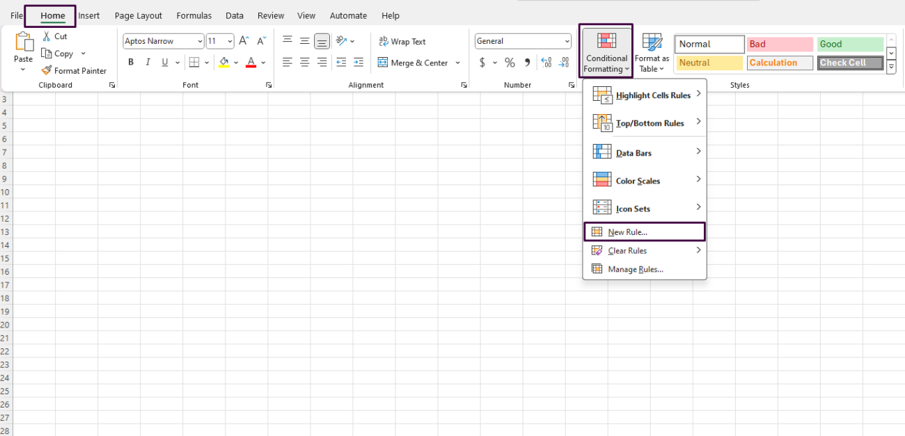
How can you Conditionally Format Dates in Excel?

Conditional formatting in Excel allows you to visually format cells based on specific conditions or criteria, making it easier to interpret data. When working with dates, conditional formatting can highlight upcoming deadlines, weekends, or past due dates, among other applications. Here’s a comprehensive guide on how to conditionally format dates in Excel.

Step 1: Open Microsoft Excel

1. Launch Microsoft Excel: Open the Excel application on your computer.
2. Open Your Workbook or Create a New One: Click on File in the top-left corner, select Open to choose an existing workbook, or click New to create a new workbook.

Step 2: Select the Range of Dates

1. Locate the Dates: Navigate to the spreadsheet that contains the dates you wish to format.
2. Select the Date Range: Click and drag to select the range of cells that contain your dates.

Step 3: Access Conditional Formatting

1. Go to the Home Tab:
   • Click on the Home tab in the Excel ribbon at the top of the screen.
2. Open Conditional Formatting:
   • Locate the Styles group within the Home tab.
   • Click on Conditional Formatting to open the drop-down menu.

Step 4: Apply Conditional Formatting to Dates

Formatting Based on Date Comparisons

1. Select New Rule:
   • From the Conditional Formatting drop-down menu, click on New Rule.
2. Choose Rule Type:
   • In the New Formatting Rule dialog box, select Format only cells that contain.
3. Set the Formatting Condition:
   • Choose Cell Value from the first drop-down menu.
   • Choose a comparison operator such as less than, equal to, or greater than.
   • Enter your specific date or use the TODAY() function for relative comparisons.

1. Format the Cells:
   • Click Format to open the Format Cells dialog box.
   • Choose your desired formatting options, such as a fill color or text style, then click OK.
2. Apply the Rule:
   • Click OK in the New Formatting Rule dialog box to apply the rule to the selected range.

Formatting for Specific Conditions

• Highlight Past Dates:
  1. Follow steps 1–3 from above.
  2. Use less than and =TODAY() to highlight all past dates.
• Highlight Future Dates:
  1. Follow steps 1–3.
  2. Use greater than and =TODAY() to format future dates.
• Highlight Weekends:
  1. Select Use a formula to determine which cells to format from the New Formatting Rule dialog box.
  2. Enter =WEEKDAY(A1,2)>5 (assuming A1 is the first cell in your range) to identify weekends.
  3. Follow steps 4–5 to apply this rule.

Step 5: Managing Conditional Formatting Rules

1. View and Edit Rules:
   • Click Conditional Formatting in the Home tab and select Manage Rules.
2. Edit or Delete Rules:
   • In the Conditional Formatting Rules Manager, select the rule you want to edit or delete.
   • Click Edit Rule to modify or Delete Rule to remove it from your spreadsheet.
3. Reorder Rules:
   • Use the arrow buttons to change the order of rules if necessary, determining which rules take precedence.

Step 6: Save Your Workbook

1. Save Your Work: Click on File and select Save or Save As to store your changes.

Looking for a budget-friendly way to get Microsoft Office? Check out our affordable Office keys and save big on premium software!