How do I Calculate the Average in Microsoft Excel?
In today’s data-driven world, being able to effectively analyze numerical data is a crucial skill. Microsoft Excel offers a range of powerful tools to aid in data analysis, and one of the most commonly used functions is calculating the average. Whether you’re a student analyzing class grades, a business professional examining financial data, or simply someone who needs to calculate the average of a set of numbers, understanding how to perform this task in Microsoft Excel is essential. In this comprehensive guide, we will take you through the step-by-step process of calculating the average in Microsoft Excel, equipping you with the knowledge to efficiently analyze and summarize numerical data for various purposes.
Calculating averages in Microsoft Excel is not only a straightforward process but also a fundamental exercise in understanding and interpreting data. Whether you’re dealing with large datasets or smaller sets of numbers, Excel provides powerful functions that enable you to effortlessly calculate averages. By learning how to utilize Excel’s built-in features, you can save time and effort while ensuring accuracy in your calculations. From finance to education, research to personal budgeting, having a solid grasp of calculating averages in Excel empowers individuals across a wide range of fields to make informed decisions based on quantitative information.
Step 1: Open Microsoft Excel and Input Data:
Begin by launching Microsoft Excel on your computer. Create a new worksheet or open an existing one where you have the dataset for which you want to calculate the average. Input the numerical data into a column or row in Excel.
Specific Command: Open Excel by searching for it in the Start menu. Click on “Blank workbook” to start a new worksheet. Enter your data into the cells.
Step 2: Select the Cell for the Average:
Click on the cell where you want the average to appear. This is typically located below or to the right of the data set you want to average.
Specific Command: Click on the cell where you want the average to be displayed.
Step 3: Use the AutoSum Function for Average:
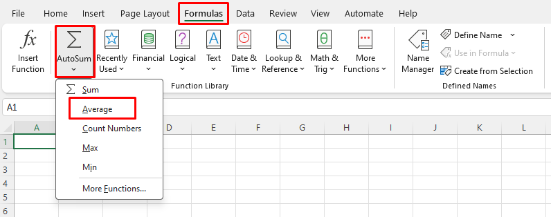
Select the cell where you want the average to be displayed. Go to the “Formulas” tab in the Excel ribbon. Click on “AutoSum” and select “Average” from the dropdown menu. Excel will automatically calculate the average of the selected data range.
Specific Command: Go to the “Formulas” tab in Excel. Click on “AutoSum” and choose “Average.”

Step 4: Manually Calculate the Average:
If you prefer to manually calculate the average, you can type the formula “=AVERAGE(” followed by selecting the range of cells containing the data you want to average. Press Enter, and Excel will calculate and display the average.
Specific Command: Type “=AVERAGE(” and select the range of cells with data. Press Enter to calculate the average.
Step 5: Review and Format the Result:
Once the average is calculated, review the result to ensure it is accurate. You can format the cell displaying the average by adjusting the font, number formatting, or adding borders to enhance readability.
By following these step-by-step instructions, you can easily calculate the average of a dataset in Microsoft Excel, empowering you to efficiently analyze numerical data and make informed decisions based on accurate calculations.
Buy a cheap Office Key directly from our website, offering a convenient and affordable way to access the essential software.

