How do I Format a Cell as Currency in Excel?
Formatting cells as currency in Excel is a fundamental skill that can help you represent monetary values accurately and professionally in your spreadsheets. Whether you are creating a budget, financial report, or invoice, correctly formatting cells as currency ensures that the numbers are displayed with the appropriate currency symbol, decimal places, and thousands separators. In this guide, we will provide you with step-by-step instructions on how to format a cell as currency in Excel, allowing you to present your financial data in a clear and visually appealing manner.
Excel provides various formatting options to customize the appearance of currency values. Our guide will cover different methods to format cells as currency, including using the currency symbol, specifying decimal places, and applying thousands separators. Additionally, we will explore advanced options, such as displaying negative numbers in red or using custom currency formats. We will also provide tips on working with currency formatting in formulas and conditional formatting. By following our guide, you will gain the knowledge and skills to confidently format cells as currency in Excel, enabling you to create professional and accurate financial spreadsheets.
Step 1: Open Microsoft Excel
- Launch Microsoft Excel on your computer.
Step 2: Select the Cell
- Select the cell or range of cells that you want to format as currency.
Step 3: Access the Format Cells Dialog Box
- Right-click on the selected cell(s) and choose “Format Cells” from the context menu.
- Alternatively, go to the “Home” tab in the Excel ribbon and click the “Format Cells” button in the “Number” group.
Step 4: Choose the Currency Category
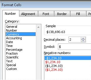
- In the “Format Cells” dialog box, go to the “Number” tab.
- Select the “Currency” category from the list on the left.

Step 5: Set the Currency Symbol
- Choose the desired currency symbol from the symbol dropdown list.
- If your desired currency symbol is not available, use the “Custom” category and input the symbol manually.
Step 6: Specify Decimal Places
- Determine the number of decimal places you want to display for your currency.
- Use the “Decimal places” dropdown to select the appropriate option.
Step 7: Choose Additional Formatting Options
- Customize the formatting options according to your preferences.
- You can adjust the symbol position, enable or disable negative number formatting, and modify other display settings.
Step 8: Apply the Currency Formatting
- Click “OK” to apply the currency formatting to the selected cell(s).
- The cell(s) will now display the chosen currency symbol and formatting.
Step 9: Apply the Formatting to Other Cells
- If you need to apply the same currency formatting to other cells, you can use the “Format Painter” icon.
- Select a cell with the desired formatting, then click the “Format Painter” icon in the “Home” tab.
- Click and drag over the cells where you want to apply the currency formatting.
Conclusion:
By following these step-by-step instructions, you can easily format cells as currency in Excel. Whether you need to work with financial data, create invoices, or simply display monetary values accurately, formatting cells as currency helps to enhance the visual representation of your data.
Get Microsoft Office from our website at the lowest price available. Get all the essential productivity tools you need at a great deal.

