How do I use the Data Validation Feature in Excel to Create a Drop-down List?

The Data Validation feature in Excel is a powerful tool that allows users to create drop-down lists, restricting the input to a predefined set of values. This feature is particularly useful when you want to ensure data consistency and accuracy, as it prevents users from entering invalid or unexpected values. With Data Validation, users can easily create custom drop-down lists, providing a user-friendly and controlled interface for data entry. In this guide, we will explore the step-by-step process of using the Data Validation feature in Excel to create drop-down lists, empowering users to enhance data integrity and streamline their data entry process.

The primary function of the Data Validation feature in Excel is to set restrictions on the type and range of data that can be entered into a cell. By creating a drop-down list through Data Validation, users can limit the choices available for a specific cell or range of cells, guiding data entry and ensuring consistent and valid data. This feature is particularly helpful in situations where you have a fixed set of options that need to be selected, such as a list of products, regions, or categories. By implementing a drop-down list, you can improve data accuracy, prevent input errors, and increase efficiency in data entry.

Step 1: Select the Cell(s):

• Open your Excel worksheet and select the cell or range where you want to create the drop-down list.

Step 2: Access the Data Validation Feature:

• Go to the “Data” tab in the Excel ribbon.
• Click on the “Data Validation” button in the “Data Tools” group.

Step 3: Define the Validation Criteria:

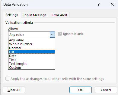
• In the Data Validation dialog box, ensure that the “Settings” tab is selected.
• Choose the “List” option from the “Allow” drop-down menu.

Step 4: Specify the Source Range:

• In the “Source” field, specify the source range for your drop-down list.
  Example: If the list is in cells A1 to A5, enter =A1:A5 in the “Source” field.

Step 5: Optional Configuration:

• Configure additional options as needed:
  • Input Message: Provide a prompt or instructions for data entry.
  • Error Alert: Define how Excel should handle invalid data inputs.

Step 6: Apply the Data Validation:

• Click on the “OK” button to apply the data validation settings to the selected cell(s).

Step 7: Testing the Drop-down List:

• Now, when you click on the drop-down arrow in the selected cell(s), the list of values from the specified range will appear.

Step 8: Modifying or Removing the Data Validation:

• To modify or delete the data validation, select the cell(s) with the drop-down list.
• Go back to the “Data” tab and click on the “Data Validation” button.
• Make the necessary changes or choose “Clear All” to remove the data validation.

By following these step-by-step instructions, you can utilize Excel’s Data Validation feature to create drop-down lists. This enables you to control and streamline data entry in your spreadsheets, ensuring accurate and efficient data collection.

If you do not have an Excel license, visit our website to obtain one from the Office Suite, offering options like Office 2016 Key, Office 2019 Key, or Office 2021 Key, tailored to your specific needs.