How to use the Grouping Function in Excel?
Excel, the widely used spreadsheet software, provides a powerful tool called the Grouping function that allows users to organize and summarize their data effectively. Whether you’re dealing with large datasets or creating complex reports, the Grouping function can streamline your workflow and enhance the clarity of your spreadsheets. In this comprehensive guide, we will walk you through the step-by-step process of utilizing the Grouping function in Excel, equipping you with the skills to efficiently group and summarize your data.
The Grouping function in Excel enables users to organize their data by grouping rows or columns based on specific criteria. By grouping related data together, you can simplify complex spreadsheets, improve data visibility, and perform summary calculations on subsets of data effortlessly. From financial analyses to data exploration, the Grouping function offers a versatile approach to managing and manipulating data within Excel.
Step 1: Open Microsoft Excel:
Launch Microsoft Excel on your computer and open the workbook where you want to use the Grouping function. If you don’t have a workbook yet, create a new one by clicking on “New Workbook” or selecting a template from the available options.
Step 2: Select the Data Range:
Identify the range of cells that contain the data you want to group. Click and drag the mouse pointer over the cells to select them. Alternatively, you can use the keyboard arrow keys to navigate to the first cell of the range, hold the Shift key, and then use the arrow keys to extend the selection.
Step 3: Access the Grouping Options:
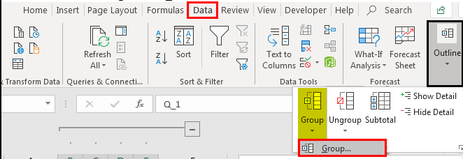
With the data range selected, go to the “Data” tab in the Excel ribbon and locate the “Outline” group. Within this group, you will find the Group and Ungroup options. Click on the “Group” button to access the grouping options.

Step 4: Group Rows or Columns:
After clicking on the “Group” button, a dialog box will appear. This box will allow you to select whether you want to group rows or columns. Choose the appropriate option based on your data structure. For example, if you have sales data by month in columns and want to group the months, select “Columns.”
Step 5: Specify the Grouping Levels:
In the same dialog box, you will have the option to specify the grouping levels. For example, if you have a dataset with sales data by year, quarter, and month, you can choose to group at each level individually or select all levels to create a hierarchical grouping. Select the appropriate levels based on your data structure.
Step 6: Grouping Options (Optional):
Excel’s Grouping function offers additional options to customize the appearance and behavior of the grouped data. Right-click on a grouped row or column, and a context menu will appear. This menu gives you options to expand or collapse the grouped data, adjust the summary functions, and even display or hide the entire group.
Step 7: Save your Workbook:
Once you have successfully grouped your data, it is crucial to save your workbook. To save, click on the “File” tab in the Excel ribbon and select the “Save” or “Save As” option. Give your workbook a name and choose a location on your computer to save it.
By following these step-by-step instructions, you can leverage the power of the Grouping function in Microsoft Excel to effectively organize and summarize your data.
Buy a cheap Office Key directly from our website, offering a convenient and affordable way to access the essential software.

