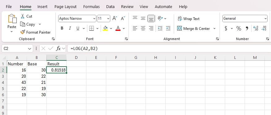
How to use the LOG Function in Excel?

The LOG function in Excel is used to find the logarithm of a number to a specified base. This function is essential for various mathematical and scientific calculations. In this step-by-step guide, we will show you how to use the LOG function effectively, including specific commands for each step.

Step 1: Open Your Excel File

1. Launch Excel: Start Microsoft Excel on your computer.
2. Open a Workbook: Go to “File” > “Open” to locate and open an existing workbook or “File” > “New” to create a new workbook.
3. Select Worksheet: Navigate to the worksheet where you want to use the LOG function.

Step 2: Identify or Enter the Number

1. Locate the Number: Identify the cell that contains the number for which you want to find the logarithm.
2. Enter the Number if Needed: If the number isn’t already in the sheet, click on an empty cell (e.g., A1) and type the number you want to use, then press Enter.

Step 3: Select the Destination Cell for the LOG Function

1. Choose the Target Cell: Click on the cell where you want to display the logarithm result (e.g., if your number is in cell A1, you might use cell B1 for the LOG function).

Step 4: Enter the LOG Function

1. Activate Formula Mode: Click on the target cell and type an equals sign = to start entering a formula.
2. Type LOG: Begin typing LOG( to start the LOG function.
3. Add Number Reference: Click on the cell containing the number (e.g., A1) or type A1 manually to reference it.
4. Specify the Base: If you have a specific base, type a comma , followed by the base number. By default, Excel uses base 10. For instance, if you are using base 2, you would enter the formula as =LOG(A1, 2).
5. Close Parenthesis: Complete the formula by typing a closing parenthesis ). Your formula should look like this: =LOG(A1, 2) for base 2 or =LOG(A1) for base 10.
6. Press Enter: Hit Enter on your keyboard to execute the function.

Step 5: Use the LOG Function on Multiple Cells (If Needed)

1. Select the Formula Cell: Click on the cell containing the LOG function (e.g., B1).
2. Drag the Fill Handle: Hover over the bottom-right corner of the cell until you see a small ‘+’ sign. Click and drag down or across to fill the formula into other cells.
3. Release Mouse Button: Release the mouse button after covering the desired range. Excel will automatically update the formulas to reference the corresponding cells.

Step 6: Verify Your Results

1. Review Logarithm Values: Check the cells where you applied the LOG function to ensure the results are as expected.
2. Adjust If Necessary: If the results are not as desired, verify the original data and ensure the formula has been entered correctly.

Step 7: Save Your Workbook

1. Save Your Work: Click “File” > “Save” or use the shortcut Ctrl + S to save your current workbook.
2. Save As New Version: To keep the original data intact, use “File” > “Save As” to create a new version of the workbook.

Get genuine Office Keys at the lowest prices exclusively on our website – unbeatable deals for all your software needs!