How to use the Row Formatting Options in Excel?
Excel is one of the most widely used spreadsheet software applications, offering a range of advanced formatting options to organize and present your data. Among these options are the row formatting features that allow users to customize the appearance of their data for easier interpretation and better organization. In this step-by-step guide, we will explore various methods to use the row formatting options in Excel, enabling you to create professional-looking spreadsheets and improve the readability and visual impact of your data.
Whether you are working with a large dataset or a small table, formatting rows can help highlight critical information, visually group related data, and create a consistent look and feel across your spreadsheet. By mastering the row formatting features of Excel, you can go beyond basic spreadsheets and create highly professional-looking reports and tables. In this guide, we will cover everything from selecting rows and accessing the formatting options to customizing the row height, giving you the tools you need to take your Excel skills to the next level. Let’s dive in and discover how to use the row formatting options in Excel.
Step 1: Open Excel and Select the Rows:
Launch Microsoft Excel on your computer and open the worksheet you want to work with. Use your mouse or keyboard to select the rows you wish to format.
Specific Commands: Double-click the Excel icon on your desktop or navigate to the program through the Start menu. Open the desired worksheet by clicking on the file name or using the “Open” option from the “File” tab. Click and drag your mouse to select specific rows or hold the Shift key while using the arrow keys to select multiple rows using the keyboard.
Step 2: Access the Formatting Options:
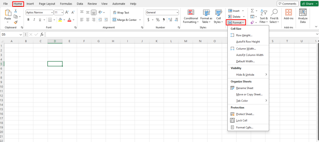
With the rows selected, go to the “Home” tab in the Excel ribbon. Locate the “Format” option in the “Cells” group and click on the small arrow next to it. A drop-down menu will appear, providing various formatting options.
Specific Commands: Click on the “Home” tab in the Excel ribbon. Find the “Format” option in the “Cells” group and click on the small arrow next to it. From the drop-down menu, select the desired formatting option for the rows.

Step 3: Apply Formatting to the Selected Rows:
Depending on the formatting option you choose, the selected rows will now be formatted accordingly. For example, you can apply different fill colors, change the font style, add borders, or adjust row height.
Specific Commands: After selecting a formatting option from the dropdown menu, the selected rows will apply the formatting instantly.
Step 4: Customize Row Height (if desired):
To adjust the height of the formatted rows, select the rows again and use the mouse to drag the row boundary line to the desired height. Alternatively, you can right-click on the row number and select “Row Height” from the context menu to enter a specific height value.
Specific Commands: To change the row height, select the rows and hover your mouse over the boundary line between two row numbers until it turns into a double-headed arrow. Click and drag the boundary line to the desired height or right-click on the row number and choose “Row Height” from the context menu to enter a specific height value.
By following these simple steps, you can easily format rows in Excel, enhancing the appearance and readability of your data. Whether you want to highlight specific rows, add borders for better organization, or adjust row height to fit your content better, Excel provides a range of options to customize and present your data effectively.
Get the best deals on purchasing the cheapest Office Key from our website.

