What is the Function of the RAND Function in Excel?
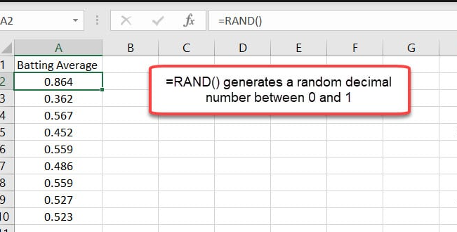
The RAND function in Excel serves as a tool for generating random numbers within a specified range. This versatile function allows users to generate random numbers in a worksheet, providing a valuable resource for simulations, statistical analysis, and other scenarios that require randomization. The RAND function generates a decimal number between 0 and 1, with each generated value being independent of any other. In this guide, we will explore the purpose and functionality of the RAND function in Excel, providing step-by-step instructions on how to effectively use this function and incorporate randomness into your spreadsheets.
The primary function of the RAND function in Excel is to produce random numbers that can be used for a variety of purposes. By using the RAND function, users can introduce unpredictability and variability into their spreadsheets. This function is commonly used in simulations to mimic real-world scenarios or in statistical analyses to generate random samples. Additionally, the RAND function can be combined with other Excel functions to perform complex calculations or create random selections.
Step 1: Open Excel and Select a Cell/Range:
- Launch Microsoft Excel and open the worksheet where you want to use the RAND function.
- Select the cell or range where you want to generate the random numbers.
Step 2: Insert the RAND Function:
- In the selected cell or range, type “=RAND()” without the quotes.
- Press Enter to execute the RAND function.

Step 3: Generate Random Numbers:
- Excel will generate a random number between 0 and 1 in the selected cell or range.
- If you want to generate a random number within a specific range, modify the formula by multiplying and adding values.
- For example, to generate a random number between 1 and 10, use the formula “=RAND()*(10-1)+1“.
Step 4: Customize the RAND Function:
- You can modify the RAND function to recalculate and generate new random numbers.
- Press F9 or go to the “Formulas” tab, and click on “Calculate Now” to recalculate the RAND function.
- Each recalculation will generate a new set of random numbers.
Step 5: Copy and Fill the RAND Function:
- If you want to generate random numbers in multiple cells or ranges, copy the RAND function.
- Select the cell or range with the RAND function, and press Ctrl+C to copy it.
- Select the target cells or ranges, and press Ctrl+V to paste the RAND function.
Step 6: Convert RAND Output to Values:
- By default, the RAND function recalculates every time you change a cell value or recalculate the worksheet.
- To convert the RAND function’s output to values, select the generated cells or ranges.
- Right-click and choose “Copy” or press Ctrl+C.
- Right-click and choose “Paste Special” or press Ctrl+Alt+V.
- In the Paste Special dialog box, select “Values” under “Paste“.
Step 7: Close Excel:
- Once you have successfully utilized the RAND function, save your Excel workbook if necessary.
- Close Excel when you are finished working.
By following these step-by-step instructions, you can use the RAND function to generate random numbers, customize the range, and convert the output to static values.
If you do not have an Excel license, visit our website to obtain one from the Office Suite, offering options like Office 2016 Key, Office 2019 Key, or Office 2021 Key, tailored to your specific needs.

