How do I use Conditional Formatting to Highlight Duplicate Values in Excel?
Conditional formatting is a powerful tool in Excel that allows users to apply formatting rules to cells based on specific conditions or criteria. One common application of conditional formatting is to highlight duplicate values in a dataset. By doing so, users can quickly identify and analyze any recurring or redundant information within their Excel spreadsheet. Whether you are managing a customer database, analyzing survey responses, or working with financial records, understanding how to use conditional formatting to highlight duplicate values can greatly improve data accuracy and streamline the decision-making process. In this guide, we will explore the step-by-step process of using conditional formatting to highlight duplicate values in Excel, empowering users to efficiently identify and manage duplicate data.
Excel’s conditional formatting feature provides a user-friendly interface for defining rules to automatically format cells based on given criteria. When it comes to identifying duplicate values, users can leverage the power of conditional formatting to visually highlight and differentiate duplicate entries from the rest of the dataset. By applying this formatting, users can easily spot any instances of repeated or redundant data points, whether they are in a single column, multiple columns, or even across different sheets.
Step 1: Open Excel and select your data
- Launch Excel and open the spreadsheet containing the data you want to analyze.
- Ensure that the data is organized properly, with the column containing the values you want to check for duplicates selected.
Step 2: Select the data range
- Click and drag to select the range of cells you want to check for duplicate values.
- Make sure to include the column header if you have one.
Step 3: Access the Conditional Formatting options
- Go to the “Home” tab on the Excel ribbon.
- Look for the “Styles” group.
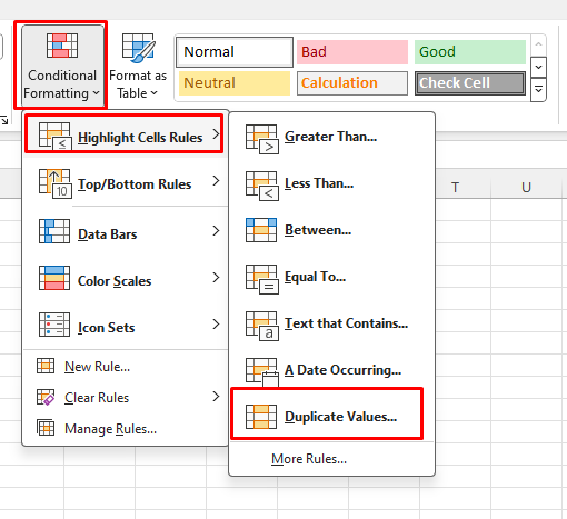
- Click on the “Conditional Formatting” button to access the dropdown menu.

Step 4: Choose the “Highlight Cells Rules” option
- From the dropdown menu, select “Highlight Cells Rules“.
- Another dropdown menu will appear.
- Select “Duplicate Values” from this menu.

Step 5: Customize the formatting for duplicate values
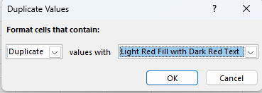
- In the “Duplicate Values” dialog box, you can choose the formatting options for the duplicate values.
- Select a format from the “Format Cells” dropdown to apply a specific style to the duplicate values.
- You can also choose to highlight the entire row or column by selecting the appropriate option.
- Adjust the formatting options based on your preference.

Step 6: Apply the Conditional Formatting
- After customizing the formatting options, click “OK” in the “Duplicate Values” dialog box.
- Excel will apply conditional formatting to the selected range, highlighting any duplicate values according to your chosen formatting style.
Step 7: Analyze the highlighted duplicate values
- Review the data and observe the duplicate values that have been highlighted.
- Use this information to analyze patterns, identify errors, or take further action based on the duplicate values.
Step 8: Updating Conditional Formatting
- If you make changes to the data in the selected range, such as adding or removing values, Excel will automatically update the conditional formatting to reflect any new duplicates.
With the Conditional Formatting feature in Excel, you can quickly and easily highlight duplicate values in your data. By following these step-by-step instructions, you can identify duplicate values, analyze patterns, and take appropriate action based on the highlighted data.
Get your Excel license from our website! Access the Office Suite with options like Office 2016, Office 2019, or Office 2021, chosen to match your needs perfectly.

