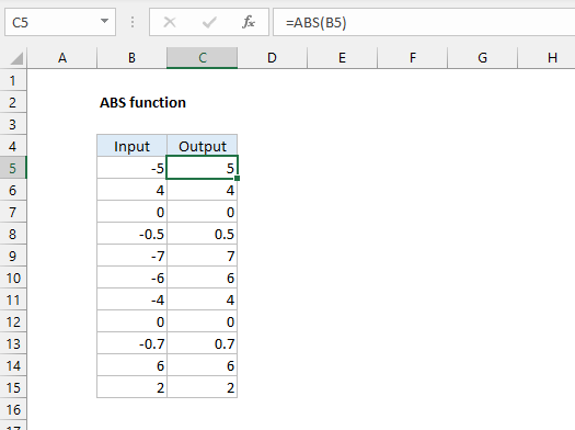
How to use the ABS Function in Excel?

The ABS function in Excel is a powerful tool for converting negative numbers into their absolute values, thereby simplifying a variety of numerical analysis tasks. This step-by-step guide will walk you through how to use the ABS function, including specific commands for each step.

Step 1: Open Your Excel File

1. Launch Excel: Start Microsoft Excel on your computer.
2. Open an Existing Workbook or Create a New One: Go to “File” > “Open” to locate and open an existing workbook or “File” > “New” to create a new workbook.
3. Select the Worksheet: Navigate to the worksheet where you want to use the ABS function.

Step 2: Identify the Cell Containing the Number

1. Locate the Number: Identify the cell that contains the number for which you want to find the absolute value.
2. Ensure Numeric Format: Check that the number is formatted as a numeric value that can be used in the ABS function.

Step 3: Select the Destination Cell for the ABS Function

1. Choose the Target Cell: Click on the cell where you want to display the absolute value (e.g., if your original number is in cell A1, you might use cell B1 for the ABS function).

Step 4: Enter the ABS Function

1. Activate Formula Mode: Click on the target cell and type an equals sign = to start entering a formula.
2. Type ABS: Begin typing ABS( to start the ABS function.
3. Add Number Reference: Click on the cell containing the number (e.g., B5) or type A1 manually to reference it.
4. Close Parenthesis: Complete the formula by typing a closing parenthesis ). Your formula should look like this: =ABS(B5).
5. Press Enter: Hit Enter on your keyboard to execute the function.

Step 5: Use the ABS Function on Multiple Cells (If Needed)

1. Select the Formula Cell: Click on the cell containing the ABS function (e.g., B1).
2. Drag the Fill Handle: Hover over the bottom-right corner of the cell until you see a small ‘+’ sign. Click and drag down or across to fill the formula into other cells.
3. Release Mouse Button: Release the mouse button after covering the desired range. Excel will automatically update the formulas to reference the corresponding cells.

Step 6: Verify Your Results

1. Review Absolute Values: Check the cells where you applied the ABS function to ensure the results are as expected.
2. Adjust If Necessary: If the results are not as desired, verify the original data and ensure the formula has been entered correctly.

Step 7: Save Your Workbook

1. Save Your Work: Click “File” > “Save” or use the shortcut Ctrl + S to save your current workbook.
2. Save As New Version: To keep the original data intact, use “File” > “Save As” to create a new version of the workbook.

Get genuine Office Keys at the lowest prices exclusively on our website – unbeatable deals for all your software needs!