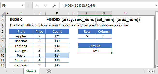
What is the Function of the INDEX Formula in Excel?

The INDEX formula in Excel plays a pivotal role in data analysis and manipulation by allowing users to retrieve specific values from a given data set. This versatile formula provides users with the ability to extract data based on certain criteria, such as row and column numbers or specific conditions met within the dataset. By utilizing the INDEX function in Excel, users can dynamically retrieve data from various locations within their spreadsheet, facilitating efficient data management and analysis. In this guide, we will explore the function and usage of the INDEX formula in Excel, providing step-by-step instructions on how to leverage this powerful tool to extract and manipulate data effectively.

The primary purpose of the INDEX formula in Excel is to retrieve specific data points or values from a selected range of cells. This function allows users to pinpoint information based on specific criteria, such as row and column numbers or conditions that the data must meet. By referencing these criteria within the INDEX formula, users can dynamically extract values from their dataset, regardless of their position or arrangement. Whether you need to extract data for calculations, create dynamic reports, or simply organize your data in a more flexible manner, the INDEX formula is an invaluable tool.

Step 1: Understanding the INDEX Formula:

• The INDEX formula returns a value or range from within a specified array.
• It requires two main arguments: the array and the row/column number indicating the position of the desired data.

Step 2: Syntax of the INDEX Formula:

• The basic syntax of the INDEX formula is: INDEX(array, row_num, [column_num]).
• The array refers to the range or table containing the data to retrieve from.
• The row_num specifies the row number from which to fetch the data.
• The optional column_num specifies the column number from which to fetch the data. If omitted, the formula returns the entire row.

Step 3: Using the INDEX Formula:

• Select the cell where you want the result to appear.
• Enter the INDEX formula using the appropriate syntax.
  Example: =INDEX(A1:D10, 3, 2) – This formula fetches the value from the third row and second column of the range A1:D10.
• Press Enter to get the result.

Step 4: Retrieving Data with INDEX and MATCH:

• INDEX can be combined with the MATCH function to search for specific values and fetch corresponding data.
• Use MATCH to find the position of a lookup value within a column or row, and pass the result as the row/column argument in the INDEX formula.

Step 5: Using INDEX with Multiple Criteria:

• In more complex scenarios, you can use INDEX with multiple criteria to retrieve data from a table based on multiple conditions.
• Combine INDEX with functions like IF, AND, and OR to determine the row or column number dynamically based on multiple criteria.

Step 6: Advanced Techniques with INDEX:

• INDEX can be used creatively to achieve various tasks, such as fetching data from different sheets, extracting multiple values, or creating dynamic ranges.
• Explore advanced techniques and functions like INDIRECT, OFFSET, or ROWS/COLUMNS in conjunction with INDEX to expand its capabilities.

The INDEX formula in Excel is a versatile tool for retrieving data based on its position within a range. By understanding its function and following these step-by-step instructions, you can effectively use the INDEX formula in your Excel spreadsheets to fetch data with precision and flexibility.

If you do not have an Excel license, visit our website to obtain one from the Office Suite, offering options like Office 2016 Key, Office 2019 Key, or Office 2021 Key, tailored to your specific needs.