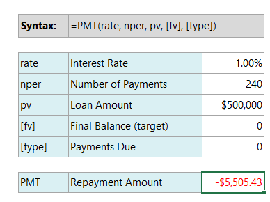
How do I use the PMT Formula in Excel to Calculate Loan Payments?
When it comes to financial planning or analyzing loan options, Excel provides users with a range of powerful formulas that can simplify complex calculations. One such formula is the PMT (Payment) formula, which enables users to calculate the periodic payments for a loan based on the loan amount, interest rate, and duration. Whether you are a financial analyst, a student, or a homeowner, understanding how to use the PMT formula in Excel can greatly assist in financial decision-making by accurately determining loan repayments and comparing different loan options. In this guide, we will delve into the step-by-step process of using the PMT formula in Excel, empowering users to calculate loan payments efficiently and make informed financial choices.
The PMT formula in Excel is designed to calculate the periodic payments required to fully repay a loan over a specified period. By inputting the loan amount, interest rate, and loan term into the formula, users can quickly obtain the monthly or annual payment amount. This feature is particularly useful when comparing loan options or budgeting for loan repayments, as it allows users to estimate the financial commitment associated with different borrowing scenarios.
Step 1: Open Excel and set up your spreadsheet
- Launch Excel and open a new or existing spreadsheet.
- Set up the necessary columns to input the loan information, such as loan amount, interest rate, and loan term.
Step 2: Input loan information
- Enter the loan amount in a cell, e.g., cell A1. Use a positive value for the loan amount.
- Enter the interest rate in another cell, e.g., cell B1. Make sure to use the per-period interest rate.
- Specify the loan term, e.g., the number of periods, in a separate cell, e.g., cell C1. Ensure the loan term aligns with the timeframe considered for interest rate calculations.
Step 3: Calculate loan payment using PMT formula
- Select a cell where you want to display the loan payment result, e.g., cell D1.
- Enter the PMT formula:
=PMT(interest_rate, loan_term, -loan_amount).- Replace “interest_rate” with the cell reference containing the interest rate value.
- Replace “loan_term” with the cell reference containing the loan term value.
- Replace “loan_amount” with the cell reference containing the loan amount value.
- Include the negative sign before the loan amount to represent outgoing payments.

Step 4: Review loan payment result
- After entering the PMT formula, Excel will calculate the loan payment based on the provided loan information.
- Verify the loan payment result in the selected cell.
Step 5: Customize formatting (if desired)
- Format the loan payment cell to display the result in your preferred currency format or decimal places.
Step 6: Modify loan information (optional)
- If you want to calculate loan payments for different scenarios, update the loan amount, interest rate, or loan term in their respective cells.
- Excel will automatically recalculate the loan payment based on the modified information.
By utilizing the PMT formula in Excel, you can effortlessly calculate loan payments based on loan amount, interest rate, and loan term. This step-by-step guide has provided you with the necessary commands and instructions to accurately calculate loan payments using the PMT formula in Excel.
Get your Excel license from our website! Access the Office Suite with options like Office 2016 License, Office 2019 License, or Office 2021 License, chosen to match your needs perfectly.

