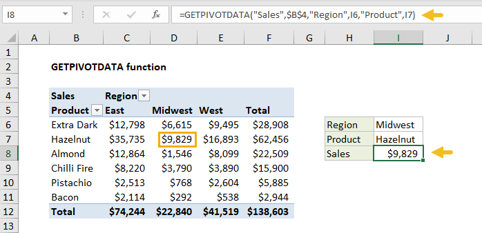
How do you use the GETPIVOTDATA Function in Excel?

The GETPIVOTDATA function is a powerful tool in Excel for extracting data from a PivotTable. It allows you to pull specific data based on the PivotTable’s layout and structure, making your reports more dynamic and accurate. In this step-by-step guide, we’ll discuss how to use the GETPIVOTDATA function effectively.

Understanding the GETPIVOTDATA Function

The syntax for the GETPIVOTDATA function is:

GETPIVOTDATA(data_field, pivot_table, [field1, item1, field2, item2], ...)

• data_field: The name of the data field you want to retrieve.
• pivot_table: A reference to any cell, range of cells, or named range in the PivotTable that contains the data you want to retrieve.
• [field1, item1, field2, item2], …: Optional pairs of field names and item names that describe the data you want to retrieve.

Step 1: Setting Up Your Excel Workbook

1. Open Excel and create a new workbook.
2. Enter your data: For our example, input the following in cells A1 to C5:Category, Product, SalesElectronics, Laptop, 1000Electronics, Mobile, 1500Furniture, Table, 200Furniture, Chair, 300
3. Create a PivotTable:
   • Select your data range (A1:C5).
   • Go to the Insert tab and click on PivotTable.
   • In the Create PivotTable dialog box, choose to place the PivotTable in a new worksheet and click OK.

Step 2: Configuring the PivotTable

1. In the PivotTable Field List:
   • Drag Category to the Rows area.
   • Drag Product to the Rows area below Category.
   • Drag Sales to the Values area.
2. The PivotTable should now display sales data organized by Category and Product.

Step 3: Using the GETPIVOTDATA Function for Basic Data Extraction

1. Select a blank cell in your worksheet where you want to display the result of the GETPIVOTDATA function, for example, E1.
2. Enter the GETPIVOTDATA formula:=GETPIVOTDATA("Sales", A3, "Category", "Electronics", "Product", "Laptop")Explanation:
   • "Sales": The field in the PivotTable you want to extract.
   • A3: A reference to any cell within the PivotTable (adjust this as per your actual PivotTable location).
   • "Category", "Electronics": Specifies we want data where the Category is Electronics.
   • "Product", "Laptop": Specifies we want data where the Product is Laptop.
3. Press Enter. The result will display the sales figure for Electronics -> Laptop, which is 1000.

Step 4: Extracting Specific Data Based on Multiple Criteria

You can use the GETPIVOTDATA function to extract data based on multiple criteria. Here’s how:

1. Select another blank cell, for example, E2.
2. Enter an advanced GETPIVOTDATA formula:=GETPIVOTDATA("Sales", A3, "Category", "Furniture", "Product", "Chair")
3. Press Enter. The result will display the sales figure for Furniture -> Chair, which is 300.

Step 5: Automating the GETPIVOTDATA Function with Dynamic References

The GETPIVOTDATA function can become even more powerful when used with dynamic cell references.

1. Select a blank cell, for example, F1, and input the text Electronics.
2. Select another blank cell, for example, G1, and input the text Mobile.
3. Select a new blank cell such as H1.
4. Enter a dynamic GETPIVOTDATA formula:=GETPIVOTDATA("Sales", A3, "Category", F1, "Product", G1)
5. Press Enter. The result will display the sales figure for Electronics -> Mobile, which dynamically updates based on the values in cells F1 and G1.

Get the cheapest Office Keys here and unlock all the premium features for a fraction of the cost!