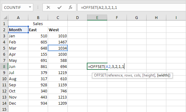
How do you use the OFFSET Function in Excel?

The OFFSET function in Excel is a powerful tool for creating dynamic ranges, summaries, and references. It’s particularly useful when you need a reference that changes based on some criteria, like the location of data or the number of rows and columns. Here is a step-by-step guide on how to use the OFFSET function effectively:

Step 1: Understand the Syntax

The basic syntax of the OFFSET function is as follows:

OFFSET(reference, rows, cols, [height], [width])

• reference: The starting point from which you want to perform your offset.
• rows: The number of rows you want to move from the starting point.
• cols: The number of columns you want to move from the starting point.
• [height] and [width] (Optional): Define the size of the range you want to return.

Step 2: Basic Example

Let’s say you have a data set in cells A1:C5, and you want to access the value that’s 2 rows down and 1 column to the right of cell A1.

Command:

=OFFSET(A1, 2, 1)

Result:
This will return the value in cell B3.

Step 3: Using OFFSET with Dynamic Ranges

One of the most powerful uses of the OFFSET function is creating dynamic named ranges that automatically adjust size based on your data.

Step 4: Creating a Dynamic Range

Suppose you have data in column A, and you want to create a dynamic range that adjusts as you add more rows.

Steps:

1. Go to the Formulas tab and select Name Manager.
2. Click New, enter a name for the range (e.g., DynamicRange), and in the Refers to field, enter: =OFFSET($A$1, 0, 0, COUNTA($A:$A), 1)
3. Click OK to save.

This dynamic range will now automatically adjust as rows are added or removed in column A.

Step 5: OFFSET with SUM Function

You can use OFFSET in conjunction with other functions like SUM to create dynamic sums.

Suppose you want to sum the first 3 values in column B, but you want this sum to shift down as new rows are added.

Command:

=SUM(OFFSET(B1, 0, 0, 3, 1))

Result:
This sums the range B1:B3.

To make it dynamic, assuming you have a numeric value for the number of rows you want to sum in cell D1:

Command:

=SUM(OFFSET(B1, 0, 0, D1, 1))

Result:
This sums the range B1 to B (whatever number is specified in D1).

Step 6: OFFSET with MATCH for Dynamic Indexing

You can combine OFFSET with the MATCH function to dynamically locate and refer to data.

Steps:

1. Suppose you want to find and return the value 2 rows down from where a specific name is located in column A.
2. First, find the row number of the specific name using MATCH: =MATCH("Specific Name", A:A, 0)
3. Then, use OFFSET to reference the value located 2 rows below that: =OFFSET(A1, MATCH("Specific Name", A:A, 0) + 1, 0)

Result:
This returns the value 2 rows below where “Specific Name” is found in column A.

Purchase genuine Office Keys on our website for unbeatable prices and instant delivery!