How to use the Data Tables and Scenarios in Microsoft Excel?
Microsoft Excel is a powerful spreadsheet program that offers a variety of features to analyze and manipulate data effectively. Two essential tools within Excel, data tables, and scenarios, provide users with valuable insights and the ability to compare multiple outcomes based on different variables. In this guide, we will explore how to utilize data tables and scenarios in Excel, enabling you to make informed decisions and gain a deeper understanding of your datasets.
Data tables in Excel allow you to perform complex calculations and analyze various scenarios by simply changing input values. Whether you need to calculate sales projections, evaluate financial models, or analyze the impact of different variables, data tables provide a dynamic and efficient solution. By following the step-by-step instructions in this guide, you will learn how to create and customize data tables, allowing you to visualize and compare data effortlessly.

Step 1: Creating a Basic Data Table:
- Open Microsoft Excel and input the data you want to use in your table into a new worksheet.
- Select the cell directly next to any row or column that includes variable data. In this example, we will use Column B to store scenarios and Column C to show the results.
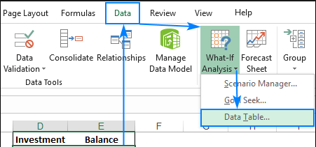
- With the empty cell selected, go to the “Data” tab in the top menu bar and click on “What-If Analysis” in the “Forecast” group.
- Click on “Data Table” in the drop-down menu and select the cell range containing the calculated formula you want to use for the table.
- In the “Row input cell” or “Column input cell” box, type the cell reference of the variable cell. For example, if we used Column B as the variable column, type “B2” to link it to the data table.
- Click “OK” to create the basic data table, which will display the calculated results for each scenario in Column C.
Step 2: Customizing the Data Table:
- With the table selected, go to the “Design” tab in the top menu bar, and choose from the preformatted styles offered in the “Table Styles” group.
- If you prefer a customized look, go to the “Table Style Options” group, and select which cells should display shading, font color, or other formatting elements.
- You can also adjust the alignment, color, and font of the data in your table by using the “Home” tab in the top menu bar.
- Finally, you can modify the variables and outcomes displayed by changing the data range referenced by the data table, or by altering the values of the variables themselves.
Step 3: Creating a Scenario:
- In addition to data tables, Excel offers a feature called “Scenarios,” which lets you compare different possible outcomes based on different sets of input values.
- Open the “Data” tab in the top menu bar and click on “What-If Analysis” in the “Forecast” group.
- Select “Scenario Manager” from the drop-down menu. In the dialog box that appears, click “Add.”
- Enter a name for the scenario and click “OK.” A new dialog box will appear, in which you can specify input cells and assign values to them.
- Click “OK” to save the scenario and return to the “Scenario Manager” dialog box.
- You can create additional scenarios by repeating these steps, which will give you an overview of how changes in input values will affect the results.
By following these simple steps, you can create and customize data tables that display a range of outcomes based on different variable inputs. You can also create scenarios that provide a comparative analysis of varying input values.
We offer the lowest prices on Office keys on our website, ensuring affordability and value for our customers.

