How do I use the Excel Data Model and Power Pivot?
The Excel Data Model and Power Pivot are powerful tools that can revolutionize the way you analyze and manage data in Excel. By incorporating these advanced features into your workflow, you can work with large datasets, create sophisticated data models, and perform complex analytical tasks with ease. This guide will provide you with a comprehensive overview of how to use the Excel Data Model and Power Pivot to unlock new capabilities and insights within your spreadsheets.
Utilizing the Excel Data Model and Power Pivot allows you to consolidate multiple data sources, create relationships between datasets, and perform advanced calculations and analysis. We will explore the process of importing data into Power Pivot, creating relationships between tables, and building robust data models to drive your analysis.
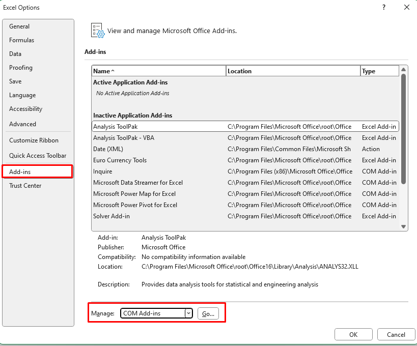
Step 1: Enable Power Pivot Add-In
Open Excel and go to the “File” tab. Click on “Options” and then select “Add-Ins.” In the Add-Ins window, select “COM Add-ins” from the Manage dropdown and click on “Go.” Check the box next to “Microsoft Office Power Pivot” and click “OK” to enable the Power Pivot add-in.

Step 2: Import Data into Power Pivot
In the Excel ribbon, click on the “Power Pivot” tab. Click on the “Manage” button to open the Power Pivot window. In the Power Pivot window, click on the “From Other Sources” button to import data from external sources like databases, Excel files, or SharePoint lists. Follow the on-screen prompts to complete the import process.
Step 3: Create Relationships between Tables
In the Power Pivot window, click on the “Diagram View” button to display the tables imported from external sources. To create relationships between tables, click and drag a column from one table to the corresponding column in another table. Repeat this process for all related tables.
Step 4: Define Calculated Columns and Measures
In the Power Pivot window, switch to the “Home” tab. To create a calculated column, click on the “Calculated Column” button and provide the formula in the formula bar. To create a measure, click on the “Measure” button and define the formula using the available functions.
Step 5: Manage Relationships and Hierarchies
To manage relationships and hierarchies, switch to the “Diagram View” in the Power Pivot window. Right-click on a relationship and select “Manage Relationships” to modify its properties. To create a hierarchy, right-click on a table column and click on “Add to Hierarchy.”
Step 6: Build PivotTables and PivotCharts
Switch back to the Excel window. In the Excel ribbon, click on the “Insert” tab. Click on the “PivotTable” button to create a new PivotTable. Select the data source and choose the fields you want to include. You can also create PivotCharts based on the PivotTable data.
Step 7: Analyze and Visualize Data
Use the PivotTable and PivotChart tools to analyze and visualize your data. Drag and drop fields into the PivotTable or PivotChart to view various data summaries and charts. Apply filters, sort data, and customize the visuals to derive insights from your data.
By following these step-by-step instructions, you can effectively use the Excel Data Model and Power Pivot to work with large datasets and perform advanced calculations in your Excel workbooks.
Shop now on our website for the best prices on Microsoft Office and boost your productivity today!

